Measures of Dispersion Class 11 Statistics Notes And Questions

Download Measures of Dispersion Class 11 notes PDF and score well in the exam. These Notes are prepared by our expert teachers at cbsencertsolutions. Class 11 Measures of Dispersion Notes assist you with overviewing the chapter in minutes. At exam time, Revision note is one of the best tips suggested by educators during exam times.

These Notes on Measure of dispersion pdf are compulsory for the Class 11 Board Exam. Measures of Dispersion Class 11 notes are exceptionally useful to revise the entire syllabus during exam time. These notes cover all significant topics and Concepts given in the section.

Please refer to Measures of Dispersion Class 11 Statistics notes and questions with solutions below. These Class 11 Statistics revision notes and important examination questions have been prepared based on the latest Statistics books for Class 11. You can go through the questions and solutions below which will help you to get better marks in your examinations.

Class 11 Statistics Measures of Dispersion Notes and Questions

1. CONCEPT AND DEFINITION OF DISPERSION
In the last two chapters, we studied Averages or Measures of Central Tendency. Average indicates representative value of the series around which other values of the series tend to converge. So that average represents the series as a whole. One may now be keen to know how far the various values of the series tend to disperse from each other, or from their average. This brings us to yet another important branch of statistical methods, viz., Measures of Dispersion. Only when we study dispersion along with average of a series that we can have a comprehensive information about the nature and composition of a statistical series. Let us take an illustration to understand the point better. The following data relates to wages paid to 5 workers in three factories, A, B and C.

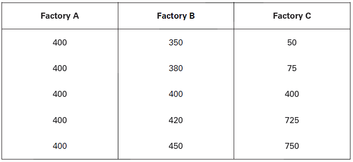
In all the three factories the arithmetic mean and median is same, i.e., 400. But in factory A, there is no variation between the average wage and the wages paid to the different labourers. In factory ‘B’, there is a small variation between average wage and wages paid to the different workers. But in factory C, there is large variation in the average wage and the wages paid to different workers. The minimum wage is Rs. 50 and maximum wage is Rs. 750. It shows that mean and median do not provide complete information about the composition and character of a series. In order to get a comprehensive picture of the series, we should study measures of dispersion as well.

How is Dispersion of the Series different from Average of the Series?

Average of the series refers to central tendency of the series. It represents behaviour of ail items in the series. But different items tend to differ from each other and from their average. Dispersion measures the extent of this difference. Or, dispersion measures the extent to which different items tend to disperse away from the central tendency.

Definition
According to Dr. Bowley, “Dispersion is the measure of the variation of the items.”

In the words of Spiegel, “The degree to which numerical data tend, to spread about an average value is called the variation or dispersion of the data.”

Objectives Related to the Measurement of Dispersion

What is the Basic Objective Related to the Measurement of Dispersion?

It is to know about the composition of the statistical series by estimating the extent to which different items of the series tend to move away from their average value or the central tendency.

Following are some specific objectives related to the measurement of dispersion:
(i) To know the variation of different values of the items from the average value of a series.
(ii) To know about the composition of a series or the dispersal of values on either sides of the central tendency.
(iii) To know the range of values (i.e., difference between the highest and the lowest value).
(iv) To compare the disparity between two or more series in order to find out the degree of variation.
(v) To know whether the central tendency truly represents the series or not.

Absolute and Relative Measures of Dispersion
There are two measures of dispersion, as discussed under:

(i) Absolute Measure
When dispersion of the series is expressed in terms of the original unit of the series, it is called absolute measure of dispersion. Thus, dispersion of price series would be expressed in terms of rupees; dispersion of weight series would be expressed in terms of kilograms; and so on. For example, if one states that the average wage of a group of the workers is Rs. 100 and dispersion of the wage is Rs. 10, one is referring to absolute dispersion. Absolute measure of dispersion is used when only one set of statistical distribution is under consideration. It cannot be used when comparison is involved across two or more sets of statistical series with different units of measurement (like ‘rupee’ in one case and ‘kilogram’ in the other).

(ii) Relative Measure
The relative measure of dispersion expresses the variability of data in terms of some relative value or percentage. Thus, if one states that 26 per cent of the people in India are below poverty line, one is referring to the relative variability of data. In such cases, absolute variability is divided by the mean value of the series or percentage of the absolute variability is determined. This measure of dispersion is used when one studies  two or more series simultaneously. Relative measure of dispersion is known as Coefficient of Dispersion.

2. METHODS OF MEASURING DISPERSION
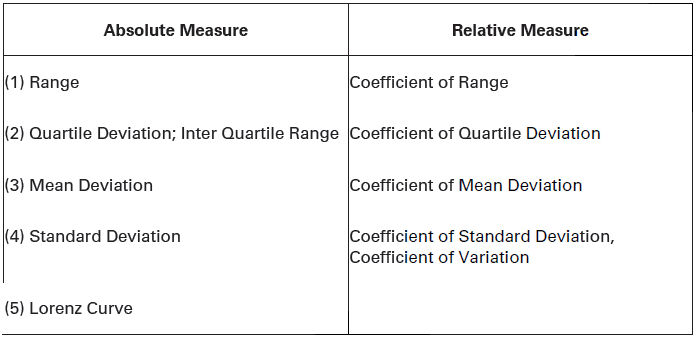
Following are the methods of absolute and relative measures of dispersion:

RANGE
It is the simplest method of measuring dispersion of data. Range is the difference between the highest value and the lowest value in a series.
Thus:

FORMULA
R = H – L
Here, R = Range; H = Highest value in the series;
L = Lowest value in the series.
To illustrate, pocket expenses of 5 students are reported to be Rs. 20, Rs. 30, Rs. 40, Rs. 50 and Rs. 100 per month. The highest value (H) in this series is Rs. 100 and the lowest
value (L) is Rs. 20. Accordingly,
R = H – L ‘
R = Rs. 100 – Rs. 20 = Rs.80
Thus, R = Rs. SO.

Why should we measure Dispersion about some particular value?
All measures of dispersion do riot measure variation about some particular value of the series. Range for example, is simply the difference between the highest and the lowest values of a statistical series, l ikewise, quartile deviation is defined as half of the difference between Q3 (third quartile) and Q1 (first quartile). But measures of dispersion like mean deviation and standard deviation are worked out as deviations from some central tendency of the statistical series. Deviations from some central tendency (or central value like mean or median) of the series offers a better picture of dispersion. Why? Because:

(i) then we can assess how precise is the central tendency as the representative value of all the observations in the series. Greater value of dispersion implies lesser representativeness of the central tendency and vice versa, and

(ii) we can precisely assess how scattered are the actual observations from their representative value. Actual observations may show both a positive variation as well as negative variation from the observed central tendency of the series. A summary measure of variation (which is what a measure of dispersion focuses on) is possible only when all the variations are duly considered.

Coefficient of Range
Range is an absolute measure of dispersion. As such it cannot be used for comparisons. To make it comparable we find its coefficient. It is the ratio between (i) the difference between the highest and lowest values of the series and (ii) the sum of the lowest and highest values of the series. It is calculated as under:

FORMULA
Coefficient of Range, CR = 𝐻−𝐿/𝐻+𝐿
(Here, CR — Coefficient of range; H = Highest value in the series; L = Lowest value in the series.)
Thus of the given illustration,
Coefficient of Range, (CR) = 100−20/100+20 = 80/120 = 0.67

Calculation of Range and Coefficient of Range for Different Types of Statistical Series
Let us understand through different illustrations how range and its coefficient are calculated for different types of statistical series.

(1) Individual Series and Range
In the individual series, range is calculated as the difference between the highest and lowest value of the series.

Illustration.
Monthly wages of workers of a factory are stated below. Find out the range and the coefficient of range.

Solution:
Range (R) = H – L
Here, H = 500; L – 50
Thus, R = 500 – 50 – 450 ,
Coefficient of Range (CR) = H−L/H+L
= 500 − 50/500 + 50
= 450/550
= 0.82
Range = 450
Coefficient of Range = 0.82.

(2) Discrete Frequency Series or Frequency Array and Range
As in the case of individual series, range of the discrete series is determined as the difference between the highest value and the lowest value of the series. Frequency of the series is not taken into account.

Illustration.
Calculate range and coefficient of range of the following series.

Note
That in the estimation of range or coefficient of range, frequency of the items is not taken into consideration.

Solution:
Here, H = 18; L = 10
Range (R) = H – L = 18-10 = 8
Coefficient of Range (CR) = H−L
H+L = 18−10
18+10 = 8
28 = 0.29
Range = 8
Coefficient of Range = 0.29.

(3) Frequency Distribution Series and Range
In case of frequency distribution series, we find the difference between lower limit of the first-class interval and upper limit of the last class interval in the series. Difference between these values would be the range of the series. That is,

FORMULA
R = Upper Limit of the Last Class Interval – Lower Limit of the First-Class Interval

Illustration.
Find out the range and the coefficient of range of the following series:

Solution:
This is an inclusive series. For the estimation of range, this must be converted into exclusive series, as below:

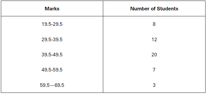
L =19.5; H = 69.5 Range (R) = 69.5 – 19.5 = 50
Coefficient of Range (CR) = 69.5−19.5/69.5+19.5 = 50/89
Range = 50

Coefficient of Range = 0.562.
Merits and Demerits of Range as a Measure of Dispersion

Merits
(1) Simple: It is a very simple measure of the dispersion of the series. It is simple to calculate as well as understand.

(2) Widely Used: Range is widely used in statistical series relating to quality control in production. Control charts are prepared on the basis of range. If the quality of goods produced is within the range prescribed in the charts then the production process is said to be under control, otherwise not. Likewise, range is a commonly used measure of dispersion in case of changes in interest rates, exchange rates and share prices.

Demerits
(1) Unstable: It is an unstable measure of dispersion. It depends upon the extreme values of the series. Any change in the extreme values or a change in the sample immediately affects the range of the series.
(2) Not Based on all Values: The calculation of range is not based on all the values of a series. It does not give importance to other values other than the extreme ones.
(3) No Knowledge of the Formation of the Series: Range gives no precise knowledge about the formation of series.
(4) Irrelevant for Open-ended Frequency Distribution: Range cannot be calculated in case of open-ended frequency distributions. It just becomes irrelevant.

Inter Quartile Range and Quartile Deviation (QD) and Their Coefficient Inter

Quartile Range
Difference between third Quartile (Q3) and first Quartile (Q₁) of a series, is called Inter Quartile Range.

FORMULA
Inter Quartile Range = Q₃ – Q₁

Quartile Deviation
Quartile Deviation is Half of Inter Quartile Range.

FORMULA
Quartile Deviation = Q₃−Q₁/2
It is also called Semi-inter Quartile Range.
Coefficient of Quartile Deviation
Coefficient of quartile deviation is calculated using the following formula:

FORMULA
Coefficient of 𝑄𝐷 = 𝑄₃−𝑄₁/2 ÷ 𝑄₃+𝑄₁/2
= Q₃ − Q₁/Q₃ + Q₁
Coefficient of Quartile Deviation = 𝑄₁−𝑄₁/𝑄₃+𝑄₁
Calculation of Quartile Deviation and Coefficient of Quartile Deviation for Different Types of Statistical Series
Through different illustrations, let us understand how quartile deviation and coefficient of quartile deviation are calculated for different statistical series.
(1) Individual Series and Quartile Deviation
In order to calculate quartile deviation in case of individual series, we first find out the values of third quartile and first quartile using the equations given on next page:
Q₁ = Size off (𝑁+1/4 )th item
Q₃ = Size of 3(𝑁+1/4 )th item
Quartile Deviation (QD) and the coefficient of QD are then calculated using the following formulae:

FORMULAE
QD = Q₃ − Q₁/2
Coefficient of QD = Q₃−Q₁/Q₃+Q1

Illustration.
Find out the quartile deviation and coefficient of quartile deviation of the following series:

𝑄₁ = SIZE OF (𝑁 + 1/4 ) TH ITEM = Size of ( 11 + 1/4 ) th item
= Size of 3rd item = 20 marks
𝑄₃ = Size of 3 ( 𝑁 + 1/4 ) th item
= Size of 3 ( 11 + 1/4 ) th item
= Size of 9th item
= 50 marks
Quartile Deviation (𝑄𝐷) = 𝑄₃−𝑄₁/2 = 50−20/2 = 15
Coefficient of Quartile Deviation = = Q₃−Q₁/Q₃+Q₁ = 50−20/50+20 = 30/70
QD = 15, Coefficient of QD = 0.43

Note
(Q₃-Q₁)/2 or quartile deviation is average of the difference between two quartiles (Q₃ and Q₁).

Illustration.
The following table shows monthly wages of 10 workers:

Calculate first, third quartiles and quartile deviation.
Solution:
Calculation of the Partition Values

Q₁ = Size of (N+1/4 ) th item= Size of (10+1/4 ) th item
= Size of 2.75th item
= Size of 2nd item+ 3/4(Size of 3rd item −Size of 2nd item)

= Rs. 150 + 3/4 (170 − 150)
Q1 = Rs. 165
Q3 = Size of 3 (N+1/4 ) th item = Size of 8.25th item
= Size of 8th item + 1/4 (Size of 9th item‐ Size of 8th item)
Q3 = Rs. 192 + 1/4 (200 − 192) = Rs. 194
QD = Q3−Q1/2 = 194−165/2 = 29/2 = 14.5

(2) Discrete Series or Frequency Array and Quartile Deviation
In a discrete series, quartile deviation is calculated by converting simple frequencies of series into cumulative frequencies. It is illustrated on next page.

Illustration.
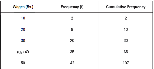
The following data shows daily wages of 199 workers of a factory. Find out quartile deviation and the coefficient of quartile deviation.

Solution:
The above series is first converted into a cumulative frequency distribution series.

Q1 = Size of (N + 1/4) th item
= Size of (199+1/4 ) th item = Size of 50th item

50th item lies in 65th cumulative frequency of the series. Wage corresponding to 65th cumulative frequency is Rs. 40 which therefore is first quartile of the wage distribution.
Likewise,

Q3 = Size of 3 (N + 1/4) th item
= Size of 3 (199+1/4 ) th item = Size of 150th item

150th item falls in 155th cumulative frequency of the series. Wage corresponding to 155th cumulative frequency is Rs. 70 which therefore is the third quartile of the series.

Quartile Deviation (𝑄𝐷) = 𝑄₃−𝑄₁/2
= 70 − 40/2
= 30/2
= 15 Coefficient of QD 𝑄𝐷 = 𝑄₃−𝑄₁/𝑄₃+𝑄₁ = 70−40/70+40 = 30/110 = 0.27

(3) Frequency Distribution Series and Quartile Deviation
Following illustration should explain the calculation of quartile deviation in frequency distribution series:

Illustration.
Find out quartile deviation of the following series:

Solution:

Q1 = Size of (N/4) th item = Size of (60/4) th item
= Size of 15 th item

15th item lies in group 40-60 and falls within 29th cumulative frequency of the series.
𝑄₁ = 𝑙₁ +𝑁4− 𝑐. 𝑓.𝑓× 𝑖

(Here, l1 = Lower limit of the class interval; N = Sum total of the frequencies; c.f. = Cumulative frequency of the class preceding the first quartile class; f = Frequency of the quartile class; i = Class interval.)

Thus,
Q₁ = 40 +60/4 −14/15 × 20
= 40 + 15 − 14/15 × 20
= 40 + 1/15 × 20
= 40 + 1.33 = 41.33

Q₃ = Size of 3 (N/4 ) th item
     = Size of 3 (60/4 ) th item
     = Size of 45th item

45th item falls within 49th cumulative frequency of the series.
Thus, Q₃ = i1 +3(N/4 )−c.f/f × i
     = 60 + 3 (60/4 ) − 29/20 × 20
     = 60 + 45 − 29/20 × 20
     = 60 +16/20 × 20
     = 60 + 16 = 76

Having known the values of Q_l and Q₃, quartile deviation (QD) is found as,
QD = Q₃−Q₁/2
     = 76 − 41.33/2
     = 34.67/2
     = 17.34
And,

Coefficient of QD = Q₃−Q₁/Q₃+Q_I
     = 76 − 41. .33/76 + 4133
     = 34.67/117.33
     = 0.30
Thus,
QD = 17.34, and Coefficient of QD = 0.30.

Merits and Demerits of Quartile Deviation
Merits

(1) Simple: It is very simple to calculate and understand.
(2) Less Effect of Extreme Values: Quartile deviation is less affected by extreme values of the series.

Demerits
(1) Not Based on all Values: The calculation of quartile deviation is not based on all
values of the series. It is, therefore, less representative.
(2) Formation of Series not known: this method does not show complete formation of
the series.
(3) Instability: The calculation of quartile deviation is significantly influenced by change
in sample of the population. Accordingly, it suffers from instability.

MEAN DEVIATION
Mean Deviation is the arithmetic average of the deviations of all the values taken from some average value (mean, median, mode) of the series, ignoring signs (+ or -) of the  deviations.
In the words of Clark and Schakde, “Mean Deviation is the Arithmetic Average of deviations of all the values taken from a statistical average (mean, median, or mode) of series. In taking deviation of values, algebraic signs + and – are not taken into consideration, that is negative deviations are also treated as positive deviations.”
Calculation of mean deviation involves the following steps:
(i) We first of all find out mean, median or mode of a series.

(ii) As a second step, we find out the deviations of different items from the (central value mean, median or mode of the series.)
These deviations are added up. While adding up these deviations positive (+) and negative (-) signs are ignored. All deviations are treated as positive.

(iii) On both sides of the deviation, from the mean, are drawn two straight lines signifying that while calculating deviation negative signs have been ignored and all deviations have been treated as positive.

(iv) Mean deviation is known by dividing the sum total of the deviation by the number of items.
Note: Deviations are often found from median value of the series. Many a time mean is also used, bur the use of Modal value is seldom made. Formula of mean deviation is as follows:

FORMULA
If deviations are taken from median, the following formula is used:
MDm = 𝛴|X − M|/N or 𝛴|dm|/N

And, if deviations are taken from arithmetic average of the series, then
MDX̅ = 𝛴|X −X̅|/N or 𝛴|dx̅|/N
(Here, MD= Mean deviation; X-M = Deviation from the median; X – X = Deviation from the arithmetic average; N = Number of items.)
Coefficient of Mean Deviation
In order to find out coefficient of mean deviation, mean deviation of the series is divided by the central tendency of the series. If the deviations are taken from arithmetic mean, the mean deviation is divided by the arithmetic mean. And, if the deviations are taken from median, the mean deviation is divided by the median. Likewise, if the deviations are taken from mode of the series, the mean deviation is divided by the mode value.
Thus,
(1) Coefficient of MD from Mean = MDx̅/X̅ = Mean Deviation/Arithmetic Mean
(2) Coefficient of MD from Median = MDm/M = Mean Deviation/Median
(3) Coefficient of MD from Mode = MD2/𝑍 = Mean Deviation/Mode

Calculation of Mean Deviation
(1) Individual Series and Mean Deviation
Following illustration should explain the calculation of mean deviation in case of individual series:

Illustration.
The data below gives wages of workers in a factory. Find out mean deviation and its coefficient.

(2) Discrete Series or Frequency Array and Mean Deviation
Following steps may be noted in the calculation of mean deviation for the discrete series:

(i) Find out central tendency of the series (mean or median) from which deviations are to be taken.

(ii) Deviations of different items in the series are taken from central tendency, and signs (+) or (-) of the deviations are ignored. It is expressed as (| dx |) or (| dm |).

(iii) Each deviation value is multiplied by the frequency facing it, and the sum of these multiples is obtained. This is expressed as Σf | d |.

(iv) Σf | d | is divided by the sum total of frequencies, that is Σf or N. The resultant value would be mean deviation. ,
Thus,

MDm = 𝛴f|dm|/N
[Here, ‘dm’ indicates that deviations are taken from median (M) of the series.]

Illustration.
Using median and arithmetic mean respectively, calculate mean deviation and its coefficient from the following data:

Solution:
(i) Calculation of Mean Deviation from Median

(a) Median or M = Size of (𝑁+1/2 )th item
= Size of (172+1/2 )th item
= Size of 36.5th item = 10
(b) Mean Deviation from Median
Or MDm = Σf|dm|/N = 148/72 = 2.05
(c) Coefficient of Mean Deviation from Median = MDm/M = 2.05/10 = 0.205

(ii) Calculation of Mean Deviation from Arithmetic Mean

(a) X = ΣfX/Σf = 708/72 = 9.83
(b) Mean Deviation from Arithmetic Mean
Or, MDλ = Σf|dx|/Σf = 150.04/72 = 2.08
(c) Coefficient of Mean Deviation from Mean =MDx/X
= 2.08/9.83 = 0.21 = 0.21

(3) Frequency Distribution Series and Mean Deviation
Continuous series are first converted into discrete series by finding mid-values of the class intervals. Afterwards, same procedure is followed for the calculation of mean deviation and its coefficient as in the case of discrete series.

Illustration.
Find out mean deviation and coefficient of mean deviation, using arithmetic mean from the following data:

Solution:

X̅ = Σfm/Σf = 2,375/75 = 31.66

Mean Deviation from Arithmetic Mean
MDX̅ = 𝛴f|dx|/𝛴f = 800 ⋅ 10/75 = 10.67

Coefficient of Mean Deviation
= MDX̅/X̅ = 10.67/31.67 = 0.34
Mean Deviation = 10.67, Coefficient of Mean Deviation = 0.34.

Illustration.
Calculate mean deviation and its coefficient from the median of the following data:

Solution:

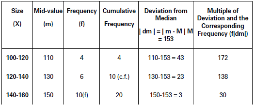
M = Size of (N/2 ) th item = Size of (33/2 ) th item
= Size of l6.5 th item
140‐160 is the Median Class Interval.

The Median is calculated as
M = l1 + N/2 − c. f/f × l
= 140 + 16. õ − 10/10 × 20
= 140 + 13 = 153

Mean Deviation from Median
MDm = Σf|dm|/Σf =661/33 = 20.03
Coefficient of Mean Deviation
= MDm/M = 20.03/153 = 0. 1309
MDn⌉ = 20.03, Cocfricient of MDm = 0.1309.
Merits and Demerits of Mean Deviation
What is the Principal Drawback of Mean Deviation as a Measure of Dispersion?
It is that all deviations from the average value of the series are taken as positive, even when some of these are actually negative.

Merits
(1) Simple: It is a very simple and easy measure of dispersion.
(2) Based on all Values: Mean deviation is based on all the items of the series. It is therefore more representative than the range or quartile deviation.
(3) Less Effect of Extreme Values: Mean deviation is less affected by extreme values than the range.

Demerits
(1) Inaccuracy: Calculation of mean deviation suffers from inaccuracy, because the *+’ or signs are ignored.
(2) Not Capable of Algebraic Treatment: Mean deviation is not capable of any further algebraic treatment.
(3) Unreliable: In case deviations are taken from mode and mode being uncertain, mean deviation also becomes uncertain and therefore, unreliable.

STANDARD DEVIATION
Standard deviation is a most satisfactory scientific method of dispersion. Accordingly, it is a widely used method in statistical analysis.

This was first used by Karl Pearson. This is sometimes called as ‘Root Mean Square Deviation’. This is generally denoted by {sigma) of the Greek language. Standard Deviation is the square root of the arithmetic mean of the squares of deviations of the items from their mean value. Standard deviation has two main features: (i) The value of its deviation is taken from arithmetic mean, (ii) Plus and minus signs of the deviations taken from the mean are not ignored. In fact, signs of the deviations become redundant once the deviations are squared. Finally, square root of the arithmetic mean of the squares of the deviation is calculated. It is this square root which is called Standard Deviation. This is always in positive value.

In the words of Spiegel, “The Standard deviation is the square root of the arithmetic mean of the squares if all deviations. Deviations being measured from arithmetic mean of the items.”

Coefficient of Standard Deviation

This is a relative measure of the dispersion of series. It is generally used whenever variation in different series is compared.

Coefficient of standard deviation is estimated by dividing the value of standard deviation by the mean of the series. Thus,

FORMULA
Coefficient of Standard Deviation = 𝜎/𝑋̅
Calculation of Standard Deviation

(1) Individual Series and Standard Deviation
There are three methods of calculating standard deviation in

case of individual series:
(i) Direct Method,
(ii) Short-cut Method, and
(iii) Step-deviation Method.

(i) Direct Method
Direct method of calculating standard deviation is most useful when mean value is in whole number. This method involves the following steps:
(a) First of all, mean value of the concerned series is determined. That is, we find out X̅ as, X̅ = ΣX/N
(b) Deviation of each item from X is determined. That is, we find the values of x as, x = X – X
(c) Each value of the deviation is squared. The sum total of the square of the deviations is obtained. That is, we find out Σx2.
(d) Σx2 is divided by the number of items (N) in the series. Square root of Σx²/N will be the standard deviation. That is, we calculate the value of √𝛴x²/N . Thus, following is the
formula for the calculation of standard deviation:
FORMULA
SD or 𝜎 = √Σx2/N or √Σ(X − X̅)²/N
(Here, σ = Standard deviation; Σx² = Sum total of the squares of deviations; X = Mean
value; X – X = Deviation from mean value; N = Number of items.)’
How Standard Deviation differs from Mean Deviation?
Standard deviation is a most satisfactory scientific method of dispersion. Accordingly, it is a widely used method in statistical analysis.

Two main differences between standard deviation and mean deviation are:
(i) In the calculation of standard deviation, deviations are taken only from the mean value of the series. On the other hand, in the calculation of mean deviation, deviations may be

taken from mean, median or mode.
(ii) In the calculation of mean deviation, signs of deviations (+) or (-) are ignored. But in the calculation of standard deviation, signs are not ignored.

Illustration.
Following are the marks obtained by 10 students of a class. Calculate standard deviation and coefficient of standard deviation.

Solution:
Calculation of Standard Deviation Using Direct Method

X̅ = ΣX/N = 110/10= 11
𝜎 = √Σx²/N = √244/10 = √24.4 = 4.94
Coefficient of SD= 𝜎/X̅
= 4.94/11 = 0.45
SD = 4.94 marks, Coefficient of SD = 0.45.

(ii) Short-cut Method

Short-cut method of calculating standard deviation involves the following steps:
(a) We take any value of the series as assumed average, generally written as A.
(b) Deviations of all the items are obtained from the assumed average. Sum total of these deviations is obtained as Σ(X – A) or Σdx.
Also, we square up the deviations and obtain their sum total as (X – A)² or Σdx².
(c) The following formula is applied to calculate the value of standard deviation:

FORMULA
𝜎 = √{Σdx2/N − (Σdx/N)²}

Illustration.
Find out standard deviation, given the following data: 8, 10, 12, 14, 16, 18, 20, 22, 24, 26

Solution:

𝜎 = √ΣDX^′2/N − (𝛴DX′/N)/² × C = √68/5 − (0/5)² × 100 = √13.6 × 100
= 3.6878 × 100 = 368.78
Standard Deviation (σ) = 368.78.

𝜎 = √Σdx²/N − (Σdx/N)²
= √420/10− (−30/10)2
= √42 − (−3)² = √33 = 5.74
Standard Deviation = 5.74.

(iii) Step-deviation Method
This method involves the following steps:
(a) We take any value of the series as assumed average.
(b) Deviations are taken from the assumed average as dx = (X-A).
(c) The deviations are divided by some common factor, as dx′ = dx/C = where C is the common factor and dx’ are step- deviations.
(d) Sum of the step-deviations is obtained. Also, step-deviations are squared and then sum total is obtained as Σdx².
(e) The following formula is applied to calculate the value of standard deviation.

FORMULA
𝜎 = √Σdx′²/N− (Σdx′/N)² × C

Illustration.
Find out standard deviation of the monthly income of 5 persons, as stated below:

Solution:

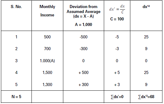
𝜎 = √ΣDX′2/N− (𝛴DX′/N)2× C
= √68/5− (0/5)2× 100
= √13.6 × 100
= 3.6878 × 100 = 368.78
Standard Deviation (σ) = 368.78.

Standard deviation in case of individual series can be calculated using the following
formula:

Illustration.
𝜎 = √ΣX/2N − (ΣX/N)²
Using electronic calculator, find out standard deviation of the following data:

Solution:
Calculation of Standard Deviation

𝜎 = √ΣX2/N − (ΣX/N)²
= √5,500/5 − (150/5)² = √1,100 − (30)²
= √1,100 − 900 = √200 = 14.14
Standard Deviation (σ) = 14.14.

(2) Discrete Series or Frequency Array and Standard Deviation
There are two methods of calculating standard deviation in discrete series:
(i) Direct Method, and
(ii) Short-cut Method.
(i) Direct Method

This method involves the following steps:

(a) We first determine mean value of the series as
X̅ = ΣfX/N

(b) Deviations of various items are obtained from the mean value as
x = X −X̅

(c) Squares of deviations are obtained as 𝑥2

(d) Squared deviations are multiplied by their corresponding frequencies, and their sum total is obtained as Σf𝑥2

(e) The following formula is applied to calculate the value of standard deviation.

FORMULA
𝜎 = √Σ𝑓x2/N
or 𝜎 = √Σf(X −X̅ )2/N

Illustration.
Find out standard deviation of the following data, using direct method:

Solution:

X̅ = ΣfX/N
= 170/17 = 10
𝜎 = √Σfx2/N
= √Σf(X − X̅)2/N
= √160/17
= √9.41
= 3.07
Standard Deviation (σ) = 3.07.

(ii) Short-cut Method
This method involves the following steps:

(a) We take any value of the series as assumed average, written as A. Generally, the value of the item with the highest frequency is taken as assumed average.

(b) Deviations of different items from assumed average are obtained as d = (X – A).

(c) Deviations are multiplied by their corresponding frequencies and then sum total is obtained as Σfd. Also, deviations are squared and multiplied by the corresponding frequencies to obtain Σfd².

(d) The following formula is applied to calculate the value of standard deviation:

FORMULA
𝜎 = √Σfd²/N − (Σfd/N)²

Illustration.

Find out standard deviation of the following data:

Solution:
Calculation of Standard Deviation (σ) in Discrete Series (Short-cut method)

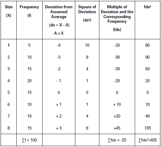
𝜎 = √Σdx²/N − (Σdx/N)²
= √435/100 − (−25/10)² = √435/100− (−1/4)²

= √435/100−1/16
= √4.29 = 2.07
Standard Deviation (σ) = 2.07.

(3) Frequency Distribution Series and Standard Deviation
Three methods are available for the calculation of standard deviation in case of frequency distribution series:
(i) Direct Method,
(ii) Short-cut Method, and
(iii) Step-deviation Method.

(i) Direct Method
This method involves the following steps:
(a) First, mean of the series (𝑋 ̅) is determined.
(b) Deviations of various mid-values are taken from the mean value, x = m – 𝑋 ̅ (Here, midvalue is m).
(c) Deviations are squared (x²) and then multiplied by their corresponding frequencies to get Σfx².
(d) Following formula is used to calculate the value of standard deviation:

FORMULA
𝜎 = √(Σ𝑓𝑥²/𝑁) or 𝜎 = √(Σ𝑓(𝑋 −𝑋 ̅ )²/𝑁)

Illustration.
Given the following series, calculate standard deviation by direct method:

Solution:

X̅ = Σfm/N = 156/24 = 6.5
𝜎 = √Σ𝑓𝑥²/𝑁
= √258/24
= √10.75 = 3.28
Standard Deviation (σ) = 3.28.

(ii) Short-cut Method
This method is the same as used in case of discrete series. The only difference is that whereas in discrete series, deviations are obtained of the actual values of the series, in case of frequency distribution series deviations are obtained of the mid-values of the class intervals. In both the cases, deviations are taken from the mean value of the series.
Thus,

FORMULA
SD or 𝜎 = √Σfdx2/N − ( Σfdx/N)²

Illustration.
Using short-cut method, calculate standard deviation of the following series:

Solution:

𝜎 = √Σfdx²/N− (𝛴fdx/N)² = √312/24− (36/24)²
= √13 − 2.25 = √10.75 = 3.28
Standard Deviation (σ) = 3.28.

(iii) Step-deviation Method
This is the most popular method of calculating standard deviation in case of frequency distribution series. It involves the following steps:
(a) Take any value as assumed average, A.
(b) Find out mid-values of the class intervals. Take deviations of the mid-values from A, expressed as ‘dx’.
(c) Divide the deviations by their common factor to get (dx/C )expressed as dx’.
(d) Multiply dx’ with the corresponding frequencies and find their sum total as Σfdx’. Also take squares of (dx’²), and multiply them by the corresponding frequencies to get Σfdx’-.
(e) Calculate the value of standard deviation, using the following formula:

FORMULA
𝜎 = √{Σfdx′²/N (Σfdx′/N)² × C}

Illustration.
Using step-deviation method, calculate standard deviation of the following series:

Solution:
Frequency Distribution Series and Standard Deviation (Step-deviation Method)

𝜎 = √Σfdx′²/N− (𝛴fdx′/N)² × C
= √369/139− (61/139)2 × 10
= √2.655 − 0.193
= √2.462 × 10
= 1.569 × 10 = 15.69
Standard Deviation (σ) = 15.69.

Illustration.
Find out standard deviation of the following data-set, using step- deviation method:

Solution:

𝜎 = √Σfdx′²/N− (Σfdx′/N)² × C
= √133/50− (−21/50)² × 20 [ Here ,C = 20]
= √2.66 − 0.1764 × 20
= √2.4836 × 20
= 1.576 × 20 = 31.52
Standard Deviation (σ) = 31.52.
Combined Standard Deviation
Just as it is possible to calculate combined mean of two or more groups, similarly the combined standard deviation of two or more groups can be calculated. The combined standard deviation of two groups is denoted by σ12 and is computed as follows:

FORMULA
𝜎12 = √{N₁𝜎₁² + N2𝜎₂² + N₁d₁² + N2d₂²}/N₁ + N₂
Where, σ_I² = Combined standard deviation;
σ_I = Standard deviation of the first group;
σ₂ = Standard deviation of the second group;
d_I = X̅
1 −X̅
1₂, d₂ =X̅
2 −X̅ 12
The above formula can be extended to calculate the standard deviation of three or more groups. For example, combined standard deviation of three groups is given by:

FORMULA
𝜎123 = √{N₁𝜎₁² + N₂𝜎₂² + N₃𝜎₃² + N₁d₁² + N₂d₂² + N₃d₃²}/N₁ + N₂ + N₃

Where, d₁ =X̅₁ −X̅₁2j; d₂ =X̅2 −X̅123; d₃ =X̅₃ −X̅123

Illustration.
Two samples of size 100 and 150 respectively have means 50 and 60 and standard deviations 5 and 6. Find the mean and standard deviation of the combined sample of size 250.

Solution:
Given: N₁ = 100, x̅₁ = 50, 𝜎1 = 5 N₂ = 150, X̅₂ = 60, 𝜎₂ = 6
Now,
X = N₁X + N₂X/N₁ + N₂
= 100 × 50 + 150 × 60/100 + 150 = 5,000 + 9,000/250
= 14,000/250 = 56
d₁ =X̅₁ −X̅₁² = 50 − 56 = −6
d₂ =X̅₂ −X̅₁² = 60 − 56 = +4
𝜎12 = √{𝑁1𝜎12 + 𝑁2𝜎22 + 𝑁1𝑑12 + 𝑁2𝑑22}/𝑁1 + 𝑁2
= √{100 × (5)2 + 150 × (6)2 + 100 × (−6)2 + 150 × (4)2/100 + 150}
= √{100 × 25 + 150 × 36 + 100 × 36 + 150 × 16/250}
= √{2,500 + 5,400+13,600 + 2,400/250}
= √{13,900/250}
= √556 = 7.46
Hence, the Combined Mean = 56 and the Combined Standard Deviation = 7.46.

Variance
Variance is another measure of dispersion. The term variance was first used by R.A. Fisher in 1918. Variance is the square of the standard deviation. Symbolically,

FORMULA
Variance = (SD)2 – σ2
Calculation of Variance
(i) Variance = Σf(X−X̅)²/N (Actual Mean Method)
(ii) Variance =Σfd₂/N − (Σfd/N )2 (Assumed Mean Method)
(iii) Variance = [Σfd′₂/N − (Σfd′/N )²] × C₂(Step-deviation Method)

Illustration.
Calculate the mean and variance from the data given below:

Solution:

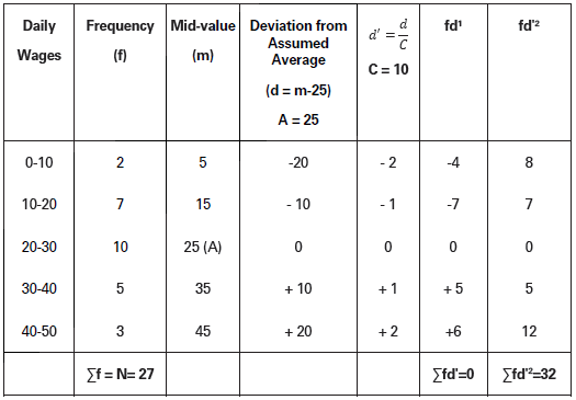
X̅ = A + Σfd′/𝛴f× C

= 25 + 0/27× 10

Variance (𝜎2) = [Σfd2/N− (Σfd′/N)2] × C2
= [32/27− (0/27)2] × 102
= σ2 = 1.185 × 100
= 118.51
Mean = 25, Variance (σ2) = 118.51.

Important
Coefficient of variation and variance are the different concepts.

Coefficient of variation is estimated as 𝜎𝑥̅ × 100; variance is simply the square of standard deviation.
(Variance = σ2)

Coefficient of Variation
Coefficient of variation is 100 times the coefficient of dispersion based on standard deviation of a statistical series. It was first used by the famous statistician Karl Pearson. That is the reason why it is called Karl Pearson’s Coefficient of Variation. In the words of Karl Pearson, “Coefficient of variation is the percentage variation in the mean, the standard deviation being considered as the total variation in the mean. ”

In order to calculate coefficient of variation, standard deviation of the series is divided by mean of the series and multiplied by 100. It is estimated using the following formula:

FORMULA
Coefficient of Variation or CV
= 𝜎/X̅× 100
= Coefficient of Standard Deviation × 100

Coefficient of Variation (CV) is 700 times the coefficient of dispersion based on standard deviation of a statistical series.

Coefficient of variation is used to compare the variability, homogeneity, stability and uniformity of two different statistical series. Higher value of coefficient of variation suggests greater degree of variability and lesser degree of stability. On the other hand, a lower value of coefficient of variation suggests lower degree of variability and higher, degree of stability, uniformity, homogeneity and consistency.

Calculation of Coefficient of Variation
(1) Individual Series and Coefficient of Variation

Illustration.
Calculate coefficient of variation of the following series:

Solution:

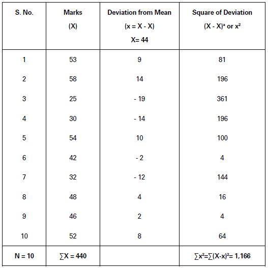
X̅ =𝛴X/N
=440/10 = 44

𝜎 = √Σx2/N
= √Σ(X −X̅)2N
= √1,166/10
= √116.6 = 10.8
CV =𝜎/X̅× 100 =10.8/44× 100= 24.55
Coefficient of Variation = 24.55.

(2) Discrete Series or Frequency Array and Coefficient of Variation
Following illustration explains the calculation of CV for discrete frequency series.

Solution:

Illustration.
Calculate coefficient of variation of the following data:

X = A + Σfdx/N = 16 + −22 50 = 1556
𝜎 = √Σfdx2/N − (Σfdx/N)2
= √452/50 − (−22/50)2
= √904 − (−0)44)2
= √904 − 01936
= √88464
= 2.97
CV = σ/x × 100 = 297/1556 × 100 = 19.09
Coefficient of Variation = 19.09.

(3) Frequency Distribution Series and Coefficient of Variation

illustration.
Calculate coefficient of variation, given the following data-set:

Solution:

X̅A + Σfdx′N× C
= 35 + 46/50 × 10 = 44.2
𝜎 = √Σfdx′2/N − (Σfdx′/N)2 × C
= √204/50− (46/50)2 × 10
= √408 − (092)2 × 10
= √408 − 08464 × 10
= √32336 × 10
= 1.798 × 10 = 17.98

CV = 𝜎/X̅ × 100
= 17.98/44.2 × 100 = 40.68
Coefficient of Variation = 40.68.

Illustration.
Batsmen X and Y score following runs in different innings they played in a test series.
Which of the two is a better scorer? Who is more consistent?

Solution:
In order to determine which of the two is a better scorer, we should compare average runs scored by two batsmen in different innings. And, in order to determine consistency of batting we should compare CV of the runs scored by the batsmen in different series.

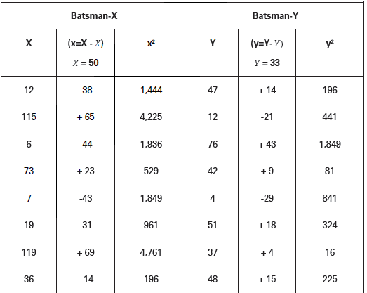
Batsman X: X = ΣX/N = 500/10 = 50

𝜎X = √Σx2/N
= √17,498/10
= √1,749.8 = 41.83
and CVx = 𝜎/𝑋̅ × 100 = 41.83/50 × 100 = 83. 11̀ 6
Batsman Y: Y = 𝛴Y/N = 330/10 = 33
𝜎Y = √Σy2/N
= √5,462/10
= √546.2 = 23.37
CVY = 𝜎/X̅ × 100X = 23.37 33 × 100 = 70.82

Since average score of X is more than that of Y, we conclude that X is a better batsman. But batting of X shows greater CV than Y. Hence, Y is relatively more consistent in batting than X.

Illustration.
Two factories A and B are located in some Industrial estate. Average wage and its standard deviation are given below separately for A and B. Find out coefficient of variation.

Solution:

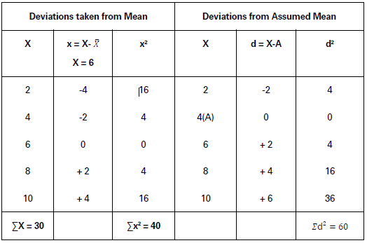
A Mathematical Property of Standard Deviation
The sum of the squares of the deviations of items from the arithmetic mean is minimum.

Merits and Demerits of Standard Deviation

Merits

(1) Based on all Values: The calculation of standard deviation is based on all the values of a series. It does not ignore any value. Accordingly, it is a comprehensive measure
of dispersion.

(2) A Certain Measure: Standard deviation is a clear and certain measure of dispersion. Therefore, it can be used in all situations.

(3) Little Effect of a change in Sample: Change in sample causes little effect on standard deviation. This is because deviation is based on all the values of a sample.

(4) Algebraic Treatment: Standard deviation is capable of further algebraic treatment.

Demerits

(1) Difficult: It is difficult to calculate and make use of standard deviation as a measure of dispersion.

(2) Importance to Extreme Values: In the calculation of standard deviation, extreme values tend to get greater importance.

LORENZ CURVE
Lorenz curve is another important measure of variability of the statistical series. This curve was first used by Max Lorenz. Hence, it is called Lorenz Curve. These curves are generally used to measure variability in the distribution of income and wealth.

Lorenz curve is a measure of deviation of actual distribution from the line of equal distribution. This is a cumulative percentage curve. The extent of deviation of the actual distribution from the equal distribution is called Lorenz coefficient. Greater the distance of

Lorenz curve from the line of equal distribution more is the inequality or variability in its series. On the other hand, closer is the Lorenz curve to the line of equal distribution,
lower will be the variability or degree of *inequality.

Construction of Lorenz Curve
Following steps are involved in the construction of a Lorenz Curve:

(i) First of all, the series is converted into a cumulative frequency series. The cumulative sum of the items (or mid-values of class intervals) is assumed to be 100 and the different items are converted into percentages of the cumulative sum. Likewise, cumulative sum of the frequencies is assumed to be 100 and different frequencies are converted into percentages of the sum of the frequencies.

(ii) Cumulative frequencies are plotted on X-axis of a graph, while cumulative items are plotted on the Y-axis.

(iii) On both axes, we start from 0 to 100 and both X and Y axes take the values from 0 to 100.

(iv) Draw a diagonal line joining the origin (0, 0) with the cumulative frequencies (100, 100). This shows equal distribution. It is, therefore, called ‘Equality Line’ or Line of Equal Distribution.

(v) Actual data are plotted on the graph and a curve is obtained by joining different points. This curve shows actual distribution.

(vi) The actual distribution curve is called Lorenz curve. Closeness of Lorenz curve to the Equal Distribution Line shows lesser variation in the distribution. Larger the gap between the actual distribution curve and the Lorenz Line, greater is the variation. If two Lorenz curves are drawn on the same graph paper, the one which is further away from the equal distribution line shows greater variation.

What is Lorenz Curve?
It is a curve that shows deviation of actual distribution (of income or wealth) from the line showing equal distribution.

Illustration.
Draw a Lorenz curve of the data given below:

Solution:

Illustration.
Show inequality in wages in two different firms using Lorenz Curve approach, given the following data:

Solution:
Estimation of Cumulative Sum and Percentage

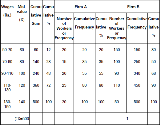
Observation: Both in firm A and firm B distribution of wages is far from equal. However, inequality is more pronounced in case of firm B than firm A as the Lorenz curve for firm B is farther away from the line of equal distribution.

Learning by doing
The following table shows number of firms in two different areas A’ and ‘B’ according to their annual profits. Present the data by way of Lorenz curve.

Make a Lorenz curve of the following data:

Application of Lorenz Curve
Lorenz Curve is a graphic measure of dispersion in a statistical series. It is a very simple measure and provides an immediate glimpse of the degree of variation in a statistical distribution from its mean value. It was first used by Prof. Lorenz for the measurement of economic inequality relating to the distribution of income and wealth across different nations or across different periods of time for the same nation. With the passage of time the application of Lorenz curve has widely spread to measure disparity of distribution

relating to various parameters like distribution of profits and wages. Briefly, Lorenz curve as a measure of dispersion is presently applied to the following parameters, viz.,
(i) distribution of income,
(ii) distribution of wealth,
(iii) distribution of wages,
(iv) distribution of profits,
(v) distribution of production, and
(vi) distribution of population.

We have provided you Class 11 Measures of Dispersion Notes Pdf Download with some important Questions and answers and there is a chance that you might observe the same kind of questions here in your exam paper too. Thus, begin learning Notes on Measure of dispersion pdf and score great marks.

We trust that you like this Measures of Dispersion Class 11 notes Pdf and it will help you to make your preparation better. Stay in contact with the page for more related stuff. If you have any questions, you might inform us by writing comments in the below box.