Please refer to Polynomials Class 9 Mathematics notes and questions with solutions below. These revision notes and important examination questions have been prepared based on the latest Mathematics books for Class 9. You can go through the questions and solutions below which will help you to get better marks in your examinations.
Class 9 Mathematics Polynomials Notes and Questions
Concept of Polynomials
Polynomials
Consider this situation involving trains.
The speed of an express train is ten less than twice that of a passenger train. If each travels for as many hours as its speed, then what is the difference between the distances travelled by them?

Let the speed of the passenger train be x km/hr.
Then, travelling time of the train = x hours
Distance travelled by it = Speed × Time = x × x = x2 km
Now, speed of the express train = (2x − 10) km/hr
Its travelling time = (2x − 10) hours
Distance travelled by it = (2x − 10) (2x − 10) = (4×2 − 40x + 100) km
Thus, required difference = 4×2 − 40x + 100 − x2 = (3×2 − 40x + 100) km
The expression 3×2 − 40x + 100 is an example of a polynomial. Different real-life problems such as the one given above can be expressed in the form of polynomials. Go through this lesson to familiarize yourself with these useful expressions.
Topics to be covered in this lesson:
♦ Identifying polynomials
♦ Constant polynomials
♦ Classification of polynomials according to the number of terms
♦ Did You Know?
♦ Ancient Babylonians developed a unique system to calculate things using formulae.
These formulae consisted of letters, mathematical operators (+, −, ×, ÷ ) and numbers. It was this system that led to the development of algebra. The word ‘algebra’ is derived from the Arabic word ‘al-jabr’ meaning ‘the reunion of broken parts’. Another Arabian connection with algebra is the Arab mathematician Muhammad ibn Musa al-Khwarizmi, whose theories greatly influenced this branch of mathematics.
♦ Did You Know?
The word ‘polynomial’ is a combination of the Greek words ‘poly’ meaning ‘many’ and ‘nomos’ meaning ‘part or portion’. Thus, a polynomial is an algebraic expression having many parts.
Different Forms of a Polynomial
♦ A polynomial can found and written in different forms. These forms are explained below.
♦ Standard form: If the terms of a polynomial are written in descending order or ascending order of the powers of the variables then the polynomial is said to be in the standard form.
♦ For example, the polynomial 3x + 15×4 − 1 − 13×2 is not in the standard form. It can be written in the standard form as 15×4 − 13×2 + 3x − 1 or −1 + 3x − 13×2+ 15×4.
♦ Index form: Observe the polynomial x6 − 2×4 − 10×3 + 5. In this polynomial, terms having x5, x2 and x are missing. These terms can be added to the polynomial with coefficient 0. Thus, the obtained polynomial will be x6 + 0x5− 2×4 − 10×3 + 0x2 + 0x + 5.
♦ The polynomial obtained on adding the missing terms is said to be in the index form.
♦ Coefficient form: When the coefficients of all the terms of a polynomial are written in a bracket by separating with comma then the polynomial is said to be written in the coefficient form.
♦ It should be noted that if a term is missing then its coefficient is taken as 0. So, it is better to write the given polynomial in the index form before wrting it in the coefficient form.
For example, to write the polynomial x6 − 2×4 − 10×3 + 5 in the coefficient form, we will first write it in the index form as x6 + 0x5− 2×4 − 10×3 + 0x2 + 0x + 5.
Now, it can be written in the coefficient form as (1, 0, −2, −10, 0, 0, 5).
Degree of Polynomial
More about Polynomials
We know that a polynomial comprises a number of terms, which may have variables or numbers or both. Also, each term can be represented with a variable having some exponent . Exponents of the variables in a given polynomial can be the same or different.
Let us consider a polynomial 2×5 + 4×2 + 9.
The terms of this polynomial and their exponents are as follows:
First term = 2×5; exponent in the first term = 5
Second term = 4×2; exponent in the second term = 2
Third term = 9 = 9×0; exponent in the third term = 0
Note that all the exponents in the above polynomial are different. These exponents help us to identify the degrees of polynomials. Polynomials are categorized based on their degrees.
In this lesson, we will learn about the degrees of polynomials and the classification of polynomials based on the same.
Whiz Kid
When a polynomial has an equals sign (=), then it becomes an equation. The maximum number of solutions of an equation is less than or equal to the degree of that equation.
The Degree of a Polynomial in more than one Variable
In case of the polynomials in one variable, the degree of a polynomial is the highest exponent of the variable in the polynomial, but what about the degree of the polynomial in more than one variable?
In this case, the sum of the powers of all variables in each term is obtained and the highest sum among all is the degree of the polynomial.
For example, find the degree of the polynomial 2xy + 3y2z + 4x2yz2 – xyz – 2×3. Let us find
the sum of the powers of all variables in each term of this polynomial.
Sum of the powers of all variables in the term 2xy = 1 + 1 = 2
Sum of the powers of all variables in the term 3y2z = 2 + 1 = 3
Sum of the powers of all variables in the term 4x2yz2 = 2 + 1 + 2 = 5
Sum of the powers of all variables in the term –xyz = 1 + 1 + 1 = 3
Sum of the powers of all variables in the term –2×3 = 3
Among all the sums, 5 is the highest and thus, the degree of the polynomial 2xy + 3y2z +
4x2yz2 – xyz – 2×3 is 5.
Similarly, we can find the degree of any polynomial in more than one variable.
Whiz Kid
If all the terms in a polynomial have the same exponent, then the expression is referred to as a homogenous polynomial.
Did You Know?
The graphs oflinear polynomials are always straight lines. This is why these polynomials are called ‘linear’ polynomials.
Values of Polynomials at Different Points
Value of a Polynomial at Different Points
What do you observe when a ball is dropped from a height? It bounces again and again until it comes to rest after some time. Also, the height to which the ball bounces keeps decreasing and then becomes zero.
Suppose a ball dropped from a certain height h bounces to two-third of that height. If this height of bounce is H, then we can say that H = 2/3 h. In this equality, the value of H changes
when the value of h undergoes a change, i.e., the value of H depends upon the value of h.
Polynomials can be described in a similar manner. When the value of the variable in a polynomial changes, the value of the polynomial also undergoes a change. This means that
the value of a polynomial depends upon the value of the variable present in it.
In this lesson, we will learn to find the value of a given polynomial at different points.
Finding the Value of a Polynomial at Different Points
Consider the polynomial, p(x) = x2 − 4x + 5. The variable here is x.
Hence, for the different values of the variable x, we get different values of the polynomial p(x).
Let us find the value of this polynomial at x = 2. We will do so by replacing x with 2 in the
given polynomial.
p(2) = 22 − 4 × 2 + 5
⇒ p(2) = 4 − 8 + 5
⇒ ∴ p(2) = 1
So, the value of the polynomial is 1 when x = 2.
Now, let us see what happens on replacing x by −3 in the given polynomial.
p(−3) = (−3)2 − 4 (−3) + 5
⇒ p(−3) = 9 + 12 + 5
⇒ ∴ p(−3) = 26
The value of the polynomial is different this time. We can see that the value of the polynomial is 26 when x = −3. This shows that the value of the polynomial changes with the change in the value of the variable in it.
Similarly, we can find the value of any polynomial for any value of the variable involved.
Did You Know?
♦ The sum of the coefficients of a polynomial p(x) is equal to p(1).
For example, let us consider a polynomial, p(x) = x2 − 4x + 5.
Here, sum of the coefficients of p(x) = p(1) = 12 − 4(1) + 5 = 2
♦ The constant coefficient of a polynomial p(x) is equal to p(0).
Let us consider the same polynomial as above.
Here, constant coefficient of p(x) = p(0) = 02 − 4(0) + 5 = 5
Whiz Kid
The plotting of the consecutive values of the variable and the polynomial on the coordinate plane gives a curve. Thus, each polynomial represents a curve.
Zeroes of Polynomials
Zero Value of a Polynomial
We know that the value of a polynomial differs according to the value of the variable in it.
For example, if p(x) is a polynomial with variable x and we put different values of x in p(x), then we will get different values of p(x). In some cases, the value of p(x) can be the same for two or more values of x. Also, in a few cases, the value of p(x) can be zero.
The values of the variable at which a polynomial becomes zero are called zeroes of the polynomial. These values are very special and useful to us. Zeroes of polynomials are used in:
Solving problems related to motion
.Solving problems related to path or Focus of a point or geometric figure
♦ Making graphs for economic data In this lesson, we will learn to check whether or not the given values are zeroes of the given polynomials. We will also learn to find the zeroes of different polynomials.
Zeroes or Roots of a Polynomial
If the value of a polynomial p(x) at x = a is zero, then a is said to be the zero or root of the polynomial p(x). Let us consider the polynomial p(x) = x2 − 5x + 6 and check its values
at
x = 1, 2 ….
p(1) = 12 − 5 × 1 + 6 = 1 − 5 + 6 = 2
p(2) = 22 − 5 × 2 + 6 = 4 − 10 + 6 = 0
p(3) = 32 − 5 × 3 + 6 = 9 − 15 + 6 = 0
Clearly, p(2) and p(3) are equal to 0; so, x = 2 and x = 3 are the zeroes or roots of the given polynomial.
The value of a constant
polynomial can never be zero. Hence, a constant polynomial has no zeroes or roots. For example, p(x) = 8 is a constant polynomial. Let us try to find the roots of this polynomial.
On replacing x with any number, we will always get 8. Suppose we replace x with 2.
Then, p(2) will still be equal to 8. This will be the case for any value of x.
Did You Know?
♦ The maximum number of roots of a polynomial is less than or equal to the degree of the polynomial. For example, the polynomial x3 − 2x + 10 has a degree 3; so, the number of roots of this polynomial will be 3, 2 or 1.
♦ Every non-constant polynomial has at least one root.
♦ A polynomial can have more than one root.
Whiz Kid
The roots of quadratic polynomials of the form ax2 + bx + c can be found by the following formula.
x = -b ± √b2 – 4ac/2a
For example, the root of x2 + 2x + 1 can be found as follows:
x = -2 ± √22 – 4(1)(1)/2(1) = -2± √4-4/2 = -2± √0/2 = -2/2 = -1
Division of Polynomials by Polynomials (Degree 1) Using Long Division Method
Dividing one number by another is something that we know well. For example, let us divide 434 by 9.
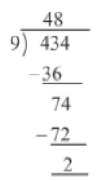
In the above division, 434 is the dividend
, 9 is the divisor
, 48 is the quotient
and 2 is the remainder
We also know how to represent any division using the division algorithm, which states that:
Dividend = Divisor × Quotient + Remainder
Thus, we can write 434 as:
434 = 9 × 48 + 2
We can divide one polynomial by another in the same way as we divide one number by another. In this lesson, we will learn to carry out the division of polynomials and verify the same using the division algorithm.
Division Algorithm
Polynomials also satisfy the division algorithm.
Consider the division of 2×2 − 9x + 4 by x − 2.
In this division, we have
Dividend = 2×2 − 9x + 4
Divisor = x − 2
Quotient = 2x − 5
Remainder = −6
Now,
Divisor × Quotient + Remainder = [(x − 2) (2x − 5)] + (−6)
= [x (2x − 5) − 2 (2x − 5)] − 6
= 2×2 − 5x − 4x +10 − 6
= 2×2 − 9x + 4
= Dividend
Thus, the given division satisfies the division algorithm, i.e,
Remainder Theorem and Its Application
Remainder Theorem
Consider two polynomials p(x) and q(x), where p(x) = 5×4 − 4×2 − 50 and q(x) = x − 2. We know how to divide p(x) by q(x) using the long division method. The result of this division will give the quotient as 5×3 + 10×2 +16x + 32 and the remainder as 14.
The long division method of finding the remainder is quite tedious. There is a simpler way to find the above remainder. This method is generalized in the form of a theorem called the remainder theorem. This theorem helps us find the remainder when a polynomial is to be divided by a linear polynomial.
In this lesson, we will study the remainder theorem and some of its applications in the form of examples.
Understanding the Remainder Theorem
Consider the division of a polynomial p(x) by a polynomial q(x), where p(x) = 5×4 − 4×2 − 50 and q(x) = x − 2. In this case, we have:
Dividend = p(x) and divisor = q(x)
On dividing p(x) by q(x) using the long division method, we get:
Quotient = 5×3 + 10×2 +16x + 32 and remainder = 14
Now, let us find the value of p(x) at x = 2.
p(2) = 5 × 24 − 4 × 22 − 50
= 5 × 16 − 4 × 4 − 50
= 80 − 16 − 50
= 14
Note how the value of p(2) is the same as the remainder obtained by the long division of p(x) by q(x). Also observe how x = 2 is a zero of the polynomial q(x).
Thus, if we replace x in the dividend with the zero (or root) of the divisor, then we get the remainder.
This method of finding the remainder is called the remainder theorem. It can be stated as follows:
For a polynomial p(x) of a degree greater than or equal to 1 and for any real number
a, if p(x) is divided by a linear polynomial x − a, then the remainder will be p(a).
Proof of the Remainder Theorem
Statement
For a polynomial p(x) of a degree greater than or equal to 1 and for any real number a, if p(x) is divided by a linear polynomial x − a, then the remainder will be p(a).
Proof
Let p(x) be a polynomial of a degree greater than or equal to 1 and a be any real number.
When divided by x − a, let p(x) leave the remainder r(x). Let q(x) be the quotient obtained.
Then, p(x) = (x − a) q(x) + r(x), where r(x) = 0 or degree r(x) < degree (x − a)
Now, x − a is a polynomial of degree 1; so, either r(x) = 0 or r(x) = constant (since a
polynomial of degree less than 1 is a constant).
Let r(x) = constant = r (say). Then, p(x) = (x − a) q(x) + r
On putting x = a, we get p(a) = (a − a) q(a) + r = 0 × q(a) + r = r
Thus, if p(x) is divided by x − a, then the remainder will be p(a).
Notes:
1) If p(x) is divided by x + a, then the remainder will be p(−a).
2) If p(x) is divided by ax − b, then the remainder will be p(b/a)
3) If p(x) is divided by ax + b, then the remainder will be p(-b/a)
Thus, when a = −9 and b = 24, the divisions of x3 + ax2 + bx − 20 by x − 5 and x −3 leave 0 and −2 respectively as the remainders.
Factor Theorem and Its Applications
Factor Theorem
We know the relation between a number and its factor. If we divide 91 by 7, then we get 13 as the quotient and zero as the remainder. In this case, we say that 7 is a factor of 91 as the remainder is zero. Now, if we divide 107 by 9, then we get 11 as the quotient and 8 as the remainder. In this case, we say that 9 is not a factor of 107 as the remainder is not zero.
Thus, the relation between a number and its factor is given as follows:
If a number is completely divisible by another number, i.e., the remainder is zero, then the second number is a factor of the first number.
Similarly, a polynomial p(x) is said to be completely divisible by a polynomial q(x) if we get zero as the remainder on dividing p(x) by q(x). In this case, we say that q(x) is a factor of p(x).
We have studied the remainder theorem that helps us to find the remainder. Similarly, we have a factor theorem that helps us to determine whether or not a polynomial is a factor of another polynomial, without actually performing the division.
In this lesson, we will study the factor theorem and solve some problems based on it.
Understanding the Factor Theorem
We can easily determine whether a polynomial q(x) is a factor of a polynomial p(x) without performing the division. This can be done by using the factor theorem, which can be stated as follows:
For a polynomial p(x) of a degree greater than or equal to 1 and for any real number c,
i) if p(c) = 0, then x − c will be a factor of p(x) and
ii) if x − c is a factor of p(x), then p(c) will be equal to zero.
Consider the polynomial, p(x) = x2 − 3x + 2.
On putting x = 2 in p(x), we get:
p(2) = 22 − 3 × 2 + 2
= 4 − 6 + 2
= 0
Thus, we can say that x − 2 is a factor of p(x), where 2 is a real number.
Proof of the Factor Theorem
Statement
For a polynomial p(x) of a degree greater than or equal to 1 and for any real number c, i) if p(c) = 0, then x − c will be a factor of p(x) and ii) if x − c is a factor of p(x), then p(c) will be equal to zero.
Proof
Let p(x) be a polynomial of a degree greater than or equal to 1 and c be any real number such that p(c) = 0. Let quotient q(x) be obtained when p(x) is divided by x − c.
i) p(c) = 0
By the remainder theorem, the remainder obtained is p(c).
⇒ p(x) = (x − c) q(x) + p(c)
⇒ p(x) = (x − c) q(x) [∵ p(c) = 0]
⇒ x − c is a factor of p(x).
ii) x − c is a factor of p(x)
⇒ When divided by x − c, p(x) leaves zero as the remainder.
However, by the remainder theorem, the remainder obtained is p(c).
⇒ p(c) = 0
Notes
1) x + c will be a factor of p(x) if p(−c) = 0
2) cx − d will be a factor of p(x) if p(d/c) = 0
3) cx + d will be a factor of p(x) if p(-d/c) = 0
4) (x − c) (x − d) will be a factor of p(x) if p(c) = 0 and p(d) = 0
Factorisation of Quadratic Polynomials Using Factor Theorem and Splitting Middle Term
Factorisation of Quadratic Polynomials
We know that 7 × 6 = 42. Here, 7 and 6 are factors of 42. Now, consider the linear polynomials
x − 2 and x + 1. On multiplying the two, we get: x (x + 1) − 2 (x + 1) = x2 + x − 2x − 2 = x2 − x − 2, which is a quadratic polynomial. So, x − 2 and x + 1 are factors of the quadratic polynomial x2 − x − 2. A quadratic polynomial can have a maximum of two factors.
In the above example, we found the quadratic polynomial from its two factors. We can also find the factors from the quadratic polynomial. This process of decomposing a polynomial into a product of its factors (which when multiplied give the original expression) is called factorisation.
There are two ways of finding the factors of quadratic polynomials viz., by applying the factor theorem and by splitting the middle term. We will discuss these methods of factorisation in this lesson and also solve some examples based on them.
Factorisation of Quadratic Polynomials Using the Factor Theorem
The factor theorem states that: For a polynomial p(x) of a degree greater than or equal to 1 and for any real number a, if p(a) = 0, then x − a will be a factor of p(x).
Consider the quadratic polynomial, p(x) = x2 − 5x + 6. To find its factors, we need to ascertain the value of x for which the value of the polynomial comes out to be zero. For this, we first determine the factors of the constant term in the polynomial, and then check the value of the polynomial at these points.
In the given polynomial, the constant term is 6 and its factors are ±1, ±2, ±3 and ±6.
Let us now check the value of the polynomial for each of these factors of 6.
p(1) = 12 − 5 × 1 + 6 = 1 − 5 + 6 = 2 ≠ 0
Hence, x − 1 is not a factor of p(x).
p(2) = 22 − 5 × 2 + 6 = 4 − 10 + 6 = 0
Hence, x − 2 is a factor of p(x).
p(3) = 32 − 5 × 3 + 6 = 9 − 15 + 6 = 0
Hence, x − 3 is also a factor of p(x).
We know that a quadratic polynomial can have a maximum two factors which are already obtained as: (x − 2) and (x − 3).
Thus, the given polynomial = p(x) = x2 − 5x + 6 = (x − 2) (x − 3)
Factorisation of Cubic Polynomial Using Factor Theorem
Factorization of Cubic Polynomials
A cubic polynomial can be written as p(x) = ax3 + bx2 + cx + d, where a, b, c and d are real numbers. We cannot factorize a cubic polynomial in the manner in which we factorize a quadratic polynomial. We use a different approach for this purpose.
A cubic polynomial can have a maximum of three linear factors. By knowing one of these factors, we can reduce it to a quadratic polynomial. Thus, to factorize a cubic polynomial, we first find a factor by the hit and trial method or by using the factor theorem, and then reduce the cubic polynomial into a quadratic polynomial. The resultant quadratic polynomial is solved by splitting its middle term or by using the factor theorem.
In this lesson, we will learn how to factorize a cubic polynomial and solve some examples related to the same.
Know More
Hit and trial method
Hit and trial method is used to find the factors or roots of a polynomial of degree more than two.
In this method, we put some value in the given polynomial to see if it satisfies the polynomial. If it does, then it is the zero of that polynomial. Using this method, we can reduce a polynomial of degree, say n, to a polynomial of degree n − 1.
Using Identity for Square of Sum of Three Terms
Algebraic Identity:
(x + y + z)2 = x2 + y2 + z2 + 2xy + 2yz + 2zx
When we solve an algebraic equation, we get the values of the variables present in it.
When an algebraic equation is valid for all values of its variables, it is called an algebraic identity.
So, an algebraic identity is a relation that holds true for all possible values of its variables.
We can use algebraic identities to expand, factorise and evaluate various algebraic expressions.
Many algebraic identities are used in mathematics. One such identity is(x + y + z)2 = x2 + y2 + z2 + 2xy + 2yz + 2zx. In this lesson, we will study this identity and solve some examples based on it.
Proof of the Identity
Let us prove the identity (x + y + z)2 = x2 + y2 + z2 + 2xy + 2yz + 2zx
We can write (x + y + z)2 as :
(a + z) 2, where a = x + y
= a2 + 2az + z2 [Using the identity (x + y) 2 = x2 + 2xy + y2]
= (x + y) 2 + 2(x + y) z + z2 (Substituting the value of a)
= x2 + 2xy + y2 + 2xz + 2yz + z2 (Using the identity (x + y) 2 = x2 + 2xy + y2)
∴ (x + y + z) 2 = x2 + y2 + z2 + 2xy + 2yz + 2zx
The above identity holds true for all values of the variables present in it. Let us verify this by substituting random values for the variables x, y and z.
If x = 2, y = 3 and z = 4, then:
(2 + 3 + 4)2 = 22 + 32 + 42 + 2 × 2 × 3 + 2 × 3 × 4 + 2 × 4 × 2
⇒ 92 = 4 + 9 + 16 + 12 + 24 + 16
⇒ 81 = 81
⇒ LHS = RHS
Thus, we see that the identity holds true for random values of the variables present in it.
Let us now use this identity to expand, factorise and evaluate various algebraic expressions.
Deriving Identity Geometrically
The identity (x + y + z)2 = x2 + y2 + z2 + 2xy + 2yz + 2zx can also be derived with the help of geometrical construction.
The steps of construction are as follows:

(1) Draw a square PQRS of side measuring (x + y + z) taking any convenient values of x, y and z.
(2) Mark two points A and B on side PQ such that l(PA) = x and l(AB) = y. Thus, l(BQ) = z.
Also, mark two points H and G on side PS such that l(PH) = x and l(HG) = y. Thus, l(GS) = z.
(3) From points A and B, draw segments AF and BE parallel to side PS and intersecting RS at F and E respectively.
(4) From points H and G, draw segments HC and GD parallel to side PQ and intersecting QR at C and D respectively.
From the figure, it can be observed that
Area of square PQRS = Sum of areas of squares PAIH, IJKL and KDRE + Sum of areas of rectangles ABJI, BQCJ, JCDK, HILG, LKEF and GLFS
⇒ (x + y + z)2 = (x2 + y2 + z2) + (xy + zx + yz + xy + yz + zx)
⇒ (x + y + z)2 = x2 + y2 + z2 + 2xy + 2yz + 2zx
Using Identities for Cube of Sum or Difference of Two Terms
Algebraic Identities:
(x + y)3 = x3 + y3 + 3xy (x + y) and (x − y)3 = x3 − y3 − 3xy (x − y)
Consider the number ‘999’. Suppose we have to calculate its cube. One way to find the cube is to multiply 999 by itself three times. However, this method is tedious and, therefore, prone to error.
Here is another way to solve the problem. Let us write 9993 as (1000 − 1)3. We have thus changed the number into the form (x − y)3. Now, the expansion of (x − y)3 will give the cube of 999. The required calculation will be easy since the values of x and y are simple numbers whose multiplication is also simple.
Thus, we see algebraic identities help make calculations simpler and less tedious. In this lesson, we will study the identities (x + y)3 = x3 + y3 + 3xy (x + y) and (x − y)3 = x3 − y3 −
3xy (x − y). We will also solve some examples based on them.
Understanding the Identities
We have the two algebraic identities as follows:
♦ (x + y)3 = x3 + y3 + 3xy (x + y) OR (x + y)3 = x3 + y3 + 3x2y + 3xy2
♦ (x − y)3 = x3 − y3 − 3xy (x − y) OR (x − y)3 = x3 − y3 − 3x2y + 3xy2
The above identities hold true for all values of the variables present in them. Let us verify this by substituting random values for the variables x and y in the first identity.
If x = 2 and y = 3, then:
(2 + 3)3 = 23 + 33 + 3 × 2 × 3 × (2 + 3)
⇒ 53 = 8 + 27 + 18 × 5
⇒ 125 = 8 + 27 + 90
⇒ 125 = 125
⇒ LHS = RHS
Thus, we see that the first identity holds true for random values of the variables present in
it. We can prove the same for the second identity as well.
Here are some other ways in which the two identities can be represented
♦ x3 + y3 = (x + y)3 − 3xy (x + y) OR x3 + y3 = (x + y) (x2 − xy + y2)
♦ x3 − y3 = (x − y)3 + 3xy (x − y) OR x3 − y3 = (x − y) (x2 + xy + y2)
Proof of the Identities:
(x + y)3 = … and x3 + y3 = …
Let us prove the identity (x + y)3 = x3 + y3 + 3x2y + 3xy2 OR (x + y)3 = x3 + y3 + 3xy (x + y)
We can write (x + y)3 as:
(x + y) (x + y)2
= (x + y) (x2 + 2xy + y2)
= x3 + 2x2y + 2xy2 + x2y + 2xy2 + y3
= x3 + y3 + 3x2y + 3xy2
∴ (x + y)3 = x3 + y3 + 3x2y + 3xy2
⇒ (x + y)3 = x3 + y3 + 3xy (x + y) … (1)
Let us prove the identity x3 + y3 = (x + y)3 − 3xy (x + y) OR x3 + y3 = (x + y) (x2 − xy + y2)
We can rewrite equation 1 as:
x3 + y3 = (x + y)3 − 3xy (x + y)
⇒ x3 + y3 =(x + y) [(x + y)2 − 3xy]
⇒ x3 + y3 = (x + y) (x2 + 2xy + y2 − 3xy)
⇒ x3 + y3 = (x + y) (x2 − xy + y2)
Proof of the Identities:
(x − y)3 = … and x3 − y3 = …
Let us prove the identity (x − y)3 = x3 − y3 − 3x2y + 3xy2 OR (x − y)3 = x3 − y3 − 3xy (x − y)
We can write (x − y)3 as:
(x − y) (x − y)2
= (x − y) (x2 − 2xy + y2)
= x3 − 2x2y + xy2 − x2y + 2xy2 − y3
= x3 − y3 − 3x2y + 3xy2
∴ (x−y)3 = x3−y3− 3x2y + 3xy2
⇒ (x − y)3 = x3 − y3 − 3xy (x − y) … (1)
Let us prove the identity x3 − y3 = (x − y)3 + 3xy (x − y) OR x3 − y3 = (x − y) (x2 + xy + y2)
We can rewrite equation 1 as:
x3 −y3 = (x−y)3 + 3xy (x−y)
⇒ x3 − y3= (x − y) [(x − y)2 + 3xy]
⇒ x3 − y3 = (x − y) (x2 − 2xy + y2 + 3xy)
⇒ x3 −y3 = (x−y) (x2 + xy + y2)
Alternate method
On using the identity p3 − q3 = (p − q) (p2 + pq + q2), where p = (2x + 5y) and q = (2x − 5y),
we get:
(2x + 5y)3 − (2x − 5y)3
= [(2x + 5y) − (2x − 5y)] [(2x + 5y)2 + (2x + 5y) (2x − 5y) + (2x − 5y)2]
= (2x + 5y − 2x + 5y) (4×2 + 20xy + 25y2 + 4×2 + 10xy − 10xy − 25y2 + 4×2 − 20xy + 25y2)
= 10y (12×2 + 25y2)
= 120x2y + 250y3
Solving Problems Using the Identity (x + y + z) (x2 + y2 + z2 − xy − yz − zx)
Algebraic Identity:
x3 + y3 + z3 − 3xyz = (x + y + z) (x2 + y2 + z2 − xy − yz − zx)
Algebraic identities help us solve problems with ease and in minimum time. Say, for example, we need to find the value of (−323 + 153 + 173). One may solve this problem by
calculating the cube of each of the given numbers and then adding and subtracting the values so obtained. This method is easy in cases where we are dealing with small numbers.
However, when big numbers are involved (as in the present case), this method proves to be tedious.
A simpler and less time-consuming way of solving the above problem is to use an appropriate algebraic identity. In the given expression, we find that −32 + 15 + 17 = 0. So, we need to state an identity under the condition x + y + z = 0.
In this lesson, we will focus on the identity x3 + y3 + z3 − 3xyz = (x + y + z) (x2 + y2 + z2 − xy − yz − zx) and its expansion under the condition x + y + z = 0. We will also solve examples based on the same.
Understanding the Identity
We have the algebraic identity as follows:
x3 + y3 + z3 − 3xyz = (x + y + z) (x2 + y2 + z2 − xy − yz − zx)
Or
x3 + y3 + z3 − 3xyz = 1/2 (x + y + z) [(x − y)2 + (y − z)2 + (z − x)2]
The above identity holds true for all values of the variables present in it. Let us verify this by substituting random values for the variables x, y and z.
If x = 1, y = 2 and z = 3, then:
13 + 23 + 33 − 3 × 1 × 2 × 3 = (1 + 2 + 3) (12 + 22 + 32 − 1 × 2 − 2 × 3 − 3 × 1)
⇒ 1 + 8 + 27 − 18 = 6 (1 + 4 + 9 − 2 − 6 − 3)
⇒ 18 = 6 × 3
⇒ 18 = 18
⇒ LHS = RHS
Thus, we see that the identity holds true for random values of the variables present in it.
Proof of the Identity
Let us prove the identity
x3 + y3 + z3 − 3xyz = (x + y + z) (x2 + y2 + z2 − xy − yz − zx)
Or
x3 + y3 + z3 − 3xyz = 1/2 (x + y + z) [(x − y)2 + (y − z)2 + (z − x)2]
We can write x3 + y3 + z3 − 3xyz as:
(x3 + y3) + z3 − 3xyz
= [(x + y)3 − 3xy(x + y)] + z3 − 3xyz
= a3 − 3axy + z3 − 3xyz, where a = x + y
= (a3 + z3) − 3axy − 3xyz
= (a + z) (a2 − az + z2) − 3xy(a + z)
= (a + z) (a2 − az + z2 − 3xy)
= (x + y + z) [(x + y)2 − (x + y)z + z2 − 3xy]
= (x + y + z) (x2 + y2 + 2xy − zx − yz + z2 − 3xy)
= (x + y + z) (x2 + y2 + z2 − xy − yz − zx)
∴ x3 + y3 + z3 − 3xyz = (x + y + z) (x2 + y2 + z2 − xy − yz − zx)
On multiplying and dividing the above expanded form by 2, we get:
1/2 × 2 (x + y + z) (x2 + y2 + z2 − xy − yz − zx)
= 1/2 (x + y + z) (2×2 + 2y2 + 2z2 − 2xy − 2yz − 2zx)
= 1/2 (x + y + z) (x2 + x2 + y2 + y2 + z2 + z2 − 2xy − 2yz − 2zx)
= 1/2 (x + y + z) (x2 + y2 − 2xy + y2 + z2 − 2yz + z2 + x2 − 2zx)
= 1/2 (x + y + z) [(x − y)2 + (y − z)2 + (z − x)2]
∴ x3 + y3 + z3 − 3xyz = 1/2 (x + y + z) [(x − y)2 + (y − z)2 + (z − x)2]
Case I of the Identity
A special case for the identity x3 + y3 + z3 − 3xyz = (x + y + z) (x2 + y2 + z2 − xy − yz − zx) is given below.
Case: When x + y + z = 0 then x3 + y3 + z3 = 3xyz.
Proof: We have,
x3 + y3 + z3 − 3xyz = (x + y + z) (x2 + y2 + z2 − xy − yz − zx)
On substituting x + y + z = 0, we obtain
x3 + y3 + z3 − 3xyz = 0 × (x2 + y2 + z2 − xy − yz − zx)
⇒ x3 + y3 + z3 − 3xyz = 0
⇒ x3 + y3 + z3 = 3xyz
Using this condition, we can factorize and find the values of many complex expressions.
Case II of the Identity
One more special case of the identity x3 + y3 + z3 − 3xyz = (x + y + z)
(x2 + y2 + z2 − xy − yz − zx) is there which is explained below.
Case: When x + y + z ≠ 0 and x3 + y3 + z3 − 3xyz = 0 then x = y = z.
Proof: We have,
x3 + y3 + z3 − 3xyz = (x + y + z) (x2 + y2 + z2 − xy − yz − zx)
On substituting x3 + y3 + z3 − 3xyz = 0, we obtain
0 = (x + y + z) (x2 + y2 + z2 − xy − yz − zx)
⇒ x2 + y2 + z2 − xy − yz − zx = 0 (x + y + z ≠ 0)
⇒ 1/2 (x + y + z) [(x − y)2 + (y − z)2 + (z − x)2]
⇒ [(x − y)2 + (y − z)2 + (z − x)2] = 0 (x + y + z ≠ 0)
Since, the sum of non negative terms such as (x − y)2, (y − z)2 and (z − x)2 is 0, each term is
0.
∴ (x − y)2 = 0, (y − z)2 = 0 and (z − x)2 = 0
⇒ x − y = 0, y − z = 0 and z − x = 0
⇒ x = y, y = z and z = x
⇒ x = y = z
This condition can be very helpful to factorize and find the values of many complex expressions.