Please refer to Organisation of Data Class 11 Statistics notes and questions with solutions below. These Class 11 Statistics revision notes and important examination questions have been prepared based on the latest Statistics books for Class 11. You can go through the questions and solutions below which will help you to get better marks in your examinations.
Class 11 Statistics Organisation of Data Notes and Questions
When an investigator collects data for an investigation, these are just raw data. Raw data are not capable of offering any meaningful conclusion. This is just like a lump of clay without any specific shape or identity. Data are to be organised before these are presented for final observations or conclusions. “Organisation of the data refers to the arrangement of figures in such a form that comparison of the mass of similar data may he facilitated and further analysis mas be possible.
An important method of organisation of data is to distribute these into different classes on the basis of their characteristics. This process is called classification of data. It involves conversion of raw data into statistical series in a manner such that some meaningful conclusions can be drawn out of them. The present chapter deals with classification of data, focusing on the conversion of raw data into various types of statistical series.
1. WHAT IS CLASSIFICATION?
There are 200 families in your locality. You have collected data regarding their income, expenditure, education, religion, size of family, etc. But this data will be of little use unless you know how many families are educated and how many are uneducated. How many families earn an income exceeding Rs. 5,000 per month and how many earn Rs. 500 or less per month.
In other words, in order to make the raw data meaningful, these must be classified on the basis of their different characteristics, such as educated families and uneducated families, rich families and poor families, etc.
Each such division of data is called Class and the process by which data is divided into different ‘classes’ on the basis of their similarity or diversity is called “Classification”. Thus, classification is the grouping of related facts into different classes. In the words of Conner, “Classification is the process of arranging things (either actually or nationally) in groups or classes according to their resemblances and affinities, and gives expression to the unity of attributes that may exist amongst a diversity of individuals This definition suggests two important features of classification:
What is the Principal Objective of Classification of Data?
It is to capture and distinctively present the diverse characteristics of data.
(i) Data are divided into different groups. For example, on the basis of education, persons may be classified as educated and uneducated.
(ii) Data are grouped or classified on the basis of their class similarities. All similar units are put in one class and as the similarity changes, class also changes. Objectives of Classification
Main objectives of Classification are as under:
(1) Brief and Simple: Main objective of classification is to present data in a form that appears to be brief and simple.
(2) Utility: Classification enhances utility of the data as it brings out similarity within the diverse set. of data.
(3) Distinctiveness: Classification renders obvious differences among the data more distinctly.
(4) Comparability: It makes data comparable and estimative.
(5) Scientific Arrangement: Classification facilitates arrangement of data in a scientific manner which increases their reliability.
(6) Attractive and Effective: Classification makes data more attractive and effective.
Characteristics of a Good Classification
(1) Comprehensiveness: Classification of the raw data should be so comprehensive that each and every item of the data gets into some group or class. No item should be left out.
(2) Clarity: Classification of the raw data into classes should be absolutely clear and simple. That is, there should be no confusion about the placement of any item in a group.
(3) Homogeneity: All items in a group or class must be homogeneous or similar to each other.
(4) Suitability: The composition of the classes must suit the objective of enquiry. For example, in order to determine the income and expenditure of the students in a school, their classification on the basis of weight or marital status would make no sense. The data must be classified on the basis of different levels of income and expenditure.
(5) Stability: A particular kind of investigation should be based on the same set of classification. This base should not change with each investigation.
(6) Elastic: Classification should be elastic. There should be a scope for change in the classification, depending on the change in purpose or objective of the study.
Basis of Classification
There may be different basis of classifying a statistical information as shown in chart below.

(1) Geographical (or Spatial) Classification: This classification of data is based on the geographical or locational differences of the data. To illustrate, data relating to the number of firms producing bicycles in India would be classified as under:
Table 1. Number of Firms Producing Bicycles in 2018 across Different Locations


(2) Chronological Classification: When data are classified on the basis of time, it is known as chronological classification. This is illustrated in the following fable 2.
Table 2 Sales of a Firm (2016-2018)

(3) Qualitative Classification: This classification is according to Qualities or Attributes of the data. For example, data may be classified on the basis of occupation, religion, level of intelligence of the population. This classification may be of two types:
(i) Simple Classification: It is called classification according to dichotomy. This is because data are divided on the basis of existence or absence of a quality. Male-female, healthy-unhealthy, educated-uneducated, are examples of dichotomy.
(ii) Manifold Classification: When classification according to quality of data involves more than one characteristic, it is called manifold classification or multiple classification. As a result of it, there may be more than two classes. To illustrate, factory workers may be classified as ‘skilled’ and ‘unskilled’. These may be further classified as literate or illiterate and still further as rural or urban. This classification may take the following form:

[Note: In qualitative classification, data are classified on the basis of a phenomenon (like honesty or beauty) which is not measurable or which cannot be expressed in terms of quantitative units like 2, 3 or 4.]
(4) Quantitative or Numerical Classification: Classification is done on the basis of numerical values of the facts. A number of classes are framed keeping in view the lowest and highest value as well as the range of values in the data. Each class of a set of data refers to a phenomenon like ‘wages’ or ‘profits’ in the automobile industry which can be expressed in figures like Indian rupees. Table 3 below is an illustration of quantitative classification:
Table 3. Annual Profit of Small-Scale Firms in the State of UP: Hypothetical Data, just for an illustration of Quantitative Classification
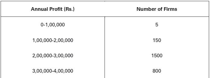
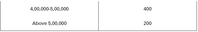
In the above classification, profit is the phenomenon under study. It is a quantifiable phenomenon. Hence, it is called quantitative classification of data.
It is important to note that the phenomenon under study (like profit in the above illustration) assumes different values over time or across different regions. When a phenomenon assumes different values it is called ‘variable’ in Statistics.
Accordingly, quantitative classification is also called ‘classification by variables.’
2. CONCEPT OF VARIABLE
A characteristic or a phenomenon which is capable of being measured and changes its value overtime is called a variable. Thus, a variable refers to that quantity which is subject to change and which can be measured by some unit. If we measure the weight of students of Class XI, then the weight of the students will be called variable. A variable may be either discrete or continuous.
Principal difference between Discrete Variable and Continuous Variable
It is that while discrete variable assumes values in complete numbers like 2, 4, S and 8,
continuous variables assume values in fractions like 2.4, 4.6 and 6.8 or values in some
range like 2-4, 4-6 etc.
(1) Discrete Variable: Discrete variables are those variables that increase in jumps or in complete numbers. For example, the number of students in Class XI could be 1, 2, 3,
10, 11, 15 or 20 etc. but cannot be 1 1 4 , 1 1 2 , 1 3 4 etc. In other words, discrete variables are expressed in terms of complete numbers, or one may simply say that values of these variables are in complete numbers as 1,2, 3 and not continuous as between 1 to 1 1 4 or a 1 3 4 and so on.
(2) Continuous Variable: Variables that assume a range of values or increase not in jumps but continuously or in fractions are called continuous variables. For example, height of the boys in a school is expressed as 5’1″, 5’2”, 5’3″, and so on. In short, while the values of discrete variables are in complete numbers (f 2, 3, etc.), values of continuous variables are in fractions (5’4″, 5’2″, etc.) or are in any range such as JO-15, 15-20, etc.
Difference between Variable and Attribute
Ordinarily, anything that varies/changes over time is taken as a variable. But not in Statistics. Colour of your hair may change over time. Is it a variable? No, not at all. Why?
Because this change cannot be numerically expressed. In Statistics, only that change of an object is taken as a variable which can be numerically expressed For example, average height of the students of Class X in the year 2005 is found to be (say) 5’6″ compared to 55″ in the previous year. Qualitative change, like a change in IQ level of the
students of Class X is called attribute’. A change in the attributes is only qualitatively expressed as good, excellent and outstanding. Qualitative changes can at best be ranked as 1, 2, 3 where 1 stands for outstanding, 2 stands for excellent and 3 stands for good.
3. RAW DATA
A mass of data in its crude form is called raw data. It is an unorganised mass of the various items. These are yet to be organised by the investigator.
To illustrate, marks obtained by 30 students of class XI in Statistics, may be expressed as in Table 4.

Data presented in this table are raw data. These are not homogeneous data or the data classified into different groups or classes with similarities. No meaningful conclusion is possible from this data. Only that data are useful to Statistics which are homogeneous. An item of the data, like the price of a commodity, income of a farmer, etc. is called observation, or value, or measure, or item, or magnitude, etc. To draw any conclusion from these data, an investigator has to first organise them. To do so, an investigator has to classify the same in the form of series.
Series: Raw data are classified in the form of series. Series refer to those data which are presented in some order and sequence. Arranging of data in different classes according
to a given order is called series. Thus, if the marks obtained by the students of Class XI are arranged according to their roll numbers in the ascending or descending order, the data so arranged would be known as statistical series. According to Horace Secrist, “4 series as used statistically may be defined as things or attributes of things arranged according to some logical order. ”
Univariate, Bivariate and Multivariate
■ ‘Uni’ means one, ‘bi’ means two.’ multi means many. Accordingly, univariate refers to a series of statistical data with one variable only, like the data on income of the households of a particular region.
■ Bivariate refers to a series of statistical data with two variables like the data on income as well as expenditure of the households of a particular region.
■ Multivariate refers to a series of statistical data with many (and more than two) variables, like the data on age, sex, education, income and expenditure of the households of a particular region.
4. CONVERSION OF RAW DATA INTO STATISTICAL SERIES
Classification of data implies conversion of raw data into statistical series. As stated earlier, classes are formed keeping in mind the nature of variables involved In the study and the range of values that the variables tend to assume.
Types of Statistical Series
Broadly, statistical series are of two types:
(1) Individual Series or Series without Frequencies, and
(2) Frequency Series or Series with Frequencies Frequency series are further divided as:
(i) Discrete Series or Frequency Array, and
(ii) Frequency Distribution or Series with Class-Intervals.

(1) Individual Series
Individual series are those series in which the items are listed singly. For example, if the marks obtained by 30 students of Class XI are listed singly, the series would be called Individual Series. In these series there is no class of the items and also there is no frequency of the items. These series may be presented in two ways:
(i) According to Serial Numbers: One way of presenting an individual series is that all the items are arranged in a serial order. Thus, marks obtained by the students may be arranged in order of their roll numbers. Data on the monthly expenses of the hostel students may be arranged in order of their room numbers. Data given in Table 4 on the marks obtained by 30 students are presented in Table 5 in order of their roll numbers.

(ii) Ascending or Descending Order of Data: The other way of presenting an individual series is a simple ascending or descending order. In the ascending order, the smallest value is placed first, while in the descending order the highest value is placed first. Tables 6 and 7 show the arrangement of data in the ascending and descending orders respectively.


Organisation of data in the form of individual series is a very simple form of presentation of data. But this method is not of much use when the number of items is very large.
(2) Frequency Series
Frequency series or series with frequencies may be of two types:
(i) Discrete Series or Frequency Array, and
(ii) Frequency Distribution.
Before we discuss these two types of series, let us understand the meaning of the following terms:
(a) Frequency: Frequency is the number of times an item occurs (or repeats itself) in the series. In other words, the number of times an item repeats itself in the population, is called the frequency of that item. For example, in Table 4, 10 has occurred 4 times. This means 4 students have secured 10 marks; or the frequency of 10 is 4.
(b) Class Frequency: The number of times an item repeats itself corresponding to a range of value (or class interval) is called class frequency. For example, if there are 4 students securing marks between 10-15, then 4 is the frequency corresponding to the class interval 10-15. Thus, 4 will be called class frequency.
(c) Tally Bars: Every time an item occurs, a tally bar, (|) is marked against that item. Corresponding to a particular class interval, each tally bar signifies ‘one’ occurrence of that item. Two tally bars would mean that the concerned item has occurred twice in the series. After every four tallies the fifth tally will cross out all the previous four tallies. Thus, making a group of five, i.e., [“HJ- This method of marking and counting is known as Four and Cross Method. To illustrate, Table 5 shows that 4 students obtained 10 marks, 5 students obtained 15 marks, 8 students obtained 20 marks, 5 students obtained 25 marks, 4 students obtained 30 marks, 2 students obtained 35 marks, 1 student obtained 40 marks and 1 student obtained 45 marks. All these frequencies have been presented in Table 8, using Four and Cross Method.
Table 8. Four and Cross Method of converting Raw Data into Frequency Series
(data as in Table 5 or 6)
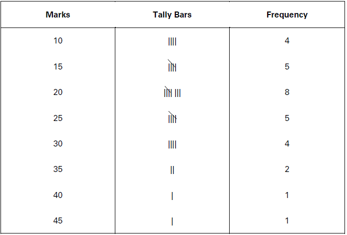
In this table, to express 8 tally bars, first of all four tally bars (||||) are marked, fifth tally bar has been marked across the four ||||. The sign |||| signifies that an item occurs five times in the series. Likewise, three tally bars are further marked |||| to make it equal to eight, i.e., |||| + | | | =8. Thus, 1 = |; 2 = ||; 3 = |||; 4 = ||||; 5 = ||||; 6 = |||| |; 7 = |||| ||; and so on.
(i) Discrete Series or Frequency Array
A discrete series or frequency array is that series in which data are presented, in a way that exact measurements of items are clearly shown. In such series there are no class intervals, and a particular item in the series is numbered rather than measured with some range.
(ii) Frequency Distribution
It is that series in which items cannot be exactly measured. The items assume a range of values and are placed within the range or limits. In other words, data are classified into different classes with a range, the range is called class intervals. Each item in the series is written against a particular class interval by way of a tally bar. The number of times an item occurs is shown as frequency against the class intervals to which that item belongs.

It is clear from above table that frequency of class interval 10-15 is 4. It means that there are 4 students who have secured marks between 10-15. Likewise, frequency of class interval 20-25 is 8 which means that there are 8 students who have secured marks between 20-25. But, it is not clear that how many students have secured 10 marks in the class interval 10-15 and how* many have secured 11 and 14 marks in the same class interval.
Size of Class
‘Size of Class’ refers to size of the class interval, or it refers to width of the class. If ‘range’ (the difference between highest value and lowest value of the series) is (say) 100 and the
number of classes is 20, then size of the class will be 100/20 = 5.
. Thus:
Size of the Class (S) = Range (r)/No.of Classes (n)
or S=r/n = 100/20 = 5 considering the above example.
Note; Size of the class must be such that all values belonging to the particular classinterval tend to converge on the mid-value of the class interval. Only then it becomes an ideal class-size. Otherwise, our result would have a high degree of statistical error.
Some Important Terms
Let us understand some important terms before a detailed study of different types of frequency distribution in the next section.
(i) Class: A range of values which incorporate a set of items is called a class. For example, 5-10, 10-15 are the classes.
(ii) Class Limits: The extreme values of a class are limits. Every class interval has two limits, lower limit and upper limit. Of the class interval 5-10 in the above example, the lower limit is 5 and the upper limit is 70.
(iii) Magnitude of a Class Interval: Magnitude of a class interval is the difference between the upper limit and the lower limit of a class. For example, in a class interval 10-15, the magnitude of the class interval would be 15 – 10 – 5. Thus, Magnitude of a Class Interval
(i) = Upper limit (l2) – Lower limit (l1)
The following formula is used to find out Class Interval.
Formula
i = l2 – l1
Where, i – magnitude of a class interval
l2 = upper limit of the class interval
l1 = lower limit of the class interval.
(iv) Mid-value: Mid-value is the average value of the upper and lower limits. It is known by adding up the upper limit and lower limit values and dividing the total by 2. Thus,
Mid-value = Upper Limit + Lower Limit/ 2
where, m = mid-value; l↑ = lower limit; l2 = upper limit.
For example, mid-value of 10-20 class interval 20+10/ 2 = 15
5. TYPES OF FREQUENCY DISTRIBUTION
Frequency Distribution is of five types:

(1) Exclusive Series
Exclusive series is that series in which every class interval excludes items corresponding to its upper limit. In this series the upper limit of one class interval is the lower limit of the next class interval. It is called exclusive series because frequencies of the upper limit of each class interval is not included in that class.
For example, in a class interval, 10-15, only such items would be included, the value of which is between 10 and 14. Any item of the value of 15 would be included in the next class interval, viz., 15-20.
(2) Inclusive Series
An inclusive series is that series which includes all items upto its upper limit. In such series, the upper limit of class interval does not repeat itself as a lower limit of the next class interval. Thus, there is a gap between the upper limit of a class interval and the lower limit of the next class interval. The gap ranges between 0.1 to 1.0. For example, 10-14, 15-19, 20-24, etc. represents an inclusive series. Thus, all the items ranging between 10-14 are included in that class interval. Likewise, all the items ranging between 15-19 would be included in that class interval.
In short, while in the exclusive series there is an overlapping of the class limits (upper class limit of one class interval being the lower class limit of the next class interval), there is no such overlapping in the inclusive series.
What is the basic difference between Exclusive Series and Inclusive Series?
In case of exclusive series upper limit of one class interval repeats itself as lower limit of the next class interval. While in case of inclusive series, it does not.
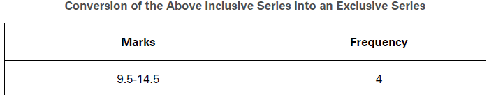
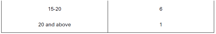
Conversion of inclusive Series into Exclusive Series
Inclusive series are used when there is some definite difference between the values of various items in the population. In the above table if a student has obtained, 14.5 or 19.5 marks these can be expressed only if the inclusive series is converted into an exclusive series. Following steps are involved in the conversion of an inclusive series into an exclusive series:
(i) First, we find the difference between the upper limit of class interval and the lower limit of the next class interval.
(ii) Half of that difference is added to the upper limit of a class interval and half is subtracted from the lower limit of the class interval.
Using these two steps, inclusive series of the above table have been converted into an exclusive series as under. Conversion of the Above Inclusive Series into an Exclusive Series

Difference between Exclusive and Inclusive Series
Main differences between exclusive and inclusive series are as under:
(i) In case of exclusive series, the upper limit of one class interval is the lower limit of the next class interval. However, in inclusive series there is generally a difference between the upper limit of one class interval and the lower limit of the other class interval.
(ii) In case of exclusive series, value of the upper limit of a class interval is not included in that class; rather it is included in the lower limit of the next class interval. On the contrary, in the case of inclusive series, value of the upper limit of a class is included in that very class interval.
(iii) Exclusive series is useful whether the value is in complete number or in decimals, but inclusive series is useful only when value is in complete number.
(iv) Counting can be done in all cases under exclusive series. However, to facilitate counting it becomes necessary to convert inclusive series into exclusive series.
(3) Open End Series
In some series, the lower class limit of the first class interval and the tipper limit of the last class interval are missing. Instead, ‘less than or below is specified in place of the lower class limit of the first class interval and ‘more than’ or above is specified in place of the upper class limit of the last class interval. Such series are called ‘Open-end’ series. Thus, an open end series is that series in which lower limit of the first class interval and (or) the upper limit of last class interval is missing. Table below shows such a series.

What is an Open-End Series?
It is that series in which
(i) lower limit of the first class interval is missing, or
(ii) upper limit of the last class interval is missing.
In order to determine the limits of the open-end class intervals, the general practice is to give same magnitude to these class intervals as is of the other class intervals in the series. However, this practice is adopted when the known magnitudes of different class intervals in the series are equal to each other. For example, in the above table since the magnitude of the class interval is the same throughout the series, first class interval will be assumed as 0-5 and last as 20-25.
(4) Cumulative Frequency Series
Cumulative frequency series is that series in which the frequencies are continuously added corresponding to each class interval in the series.
Let us proceed with an illustration of converting Simple Frequency Series into a Cumulative Frequency Series. Here is a simple frequency series.
Illustration.
Simple Frequency Series

There are two ways of converting this series into cumulative frequency series. These are:
(i) Cumulative frequencies may be expressed on the basis of upper limits of the class intervals, e.g., less than 10, less than 15, less than 20, when the class intervals are 5- 10, 10-15 and 15-20.
(ii) Cumulative frequencies may be expressed on the basis of lower-class limits of the class intervals, e.g., more than 5, more than 10, more than 15, when the class intervals are 5-10, 10-15 and 15-20.
Thus, when a frequency distribution is to be converted into a cumulative frequency distribution, the cumulative frequencies would correspond to either the lower-class limits or the upper-class limits of the class intervals in a series. Accordingly, the class intervals would get converted into ‘less than’ or ‘more than’ values. Following is an example of how’ a frequency distribution is converted into a cumulative frequency distribution.
Cumulative Frequency Series

Conversion of Cumulative Frequency Series into Simple Frequency Series
Cumulative Frequency Series may be converted into Simple Frequency Series. Following illustration explains this process:
Illustration.
Convert the following cumulative frequency series into a simple frequency series.
4 students obtained less than 10 marks
20 students obtained less than 20 marks
40 students obtained less than 30 marks
48 students obtained less than 40 marks
50 students obtained less than 50 marks
Solution:
Conversion of a Cumulative Frequency Series into a Simple Frequency Series

(5) Mid-values Frequency Series
Mid-values frequency series are those series in which we have only mid-values of the class intervals and the corresponding frequencies.

Such series may be converted into simple frequency series using the following method:
(i) First, mutual difference between mid-values (i) is determined; and (ii) Second, the difference so obtained is reduced to half (1
2 𝑖) which when deducted from the mid-value
gives lower limit of the class interval and when added to the mid-value gives the
corresponding upper limit.
Thus, Lower limit: 𝑙1 = 𝑚 − 1-2 𝑖
Upper limit: 𝑙2 = 𝑚 + 1-2 𝑖
where, m = mid-value; i = difference between mid-values; l1 — lower limit and l2 = upper limit.
In the above frequency series with raid-values, the mutual difference between midvalues
(i) = 15 – 5 = 10. Half of it is 5. Deducting 5 from each mid-value we get lower limits and adding 5 to each mid-value we get the corresponding upper limits. Following table shows the process of this conversion.
Conversion of a Series with Mid-values into a Series with Class Intervals
Illustration.

Class mid-values of a frequency distribution of marks in economics of a group of students in Class XI are given as 25, 32, 39, 46, 53 and 60.
Find the size of the class interval and class limits.
Solution:
Size of class interval = Mutual difference between mid-values
= 32 – 25 = 39 – 32 = 46 – 39 – … = 60-53
= 7
Thus, the size of the class is 7.
Given the size of the class as 7 and mid-values of classes as 25, 32, 39, 46, 53 and 60, we can now obtain the class limits by using the following formulae:
Lower limit: 𝑙1 = 𝑚 − 1-2 𝑖
Upper limit: 𝑙2 = 𝑚 + 1-2 𝑖
where, m = mid-values; i — difference between mid-values or the size of class.
Accordingly, the class limits of the first class will be:
𝑙1 = 25 − 1/2 × 7 = 25 − 3.5 = 21.5
𝑙2 = 25 +1/2
× 7 = 25 + 3.5 = 28.5
and so on.
Thus, the various classes with class limits are given as: